Van Allen Probes (RBSP)
The routines in this module can be used to load and process data (in case of RBSPICE) from the Van Allen Probes (RBSP) mission.
Electric and Magnetic Field Instrument Suite and Integrated Science (EMFISIS)
- pyspedas.projects.rbsp.emfisis(trange=['2018-11-5', '2018-11-6'], probe='a', datatype='magnetometer', level='l3', cadence='4sec', coord='sm', wavetype='waveform', prefix='', suffix='', force_download=False, get_support_data=False, varformat=None, varnames=[], downloadonly=False, notplot=False, no_update=False, time_clip=False)[source]
This function loads data from the Electric and Magnetic Field Instrument Suite and Integrated Science (EMFISIS) instrument
- For information on the EMFISIS data products, see:
https://emfisis.physics.uiowa.edu/data/level_descriptions https://emfisis.physics.uiowa.edu/data/L2_products
- Parameters:
trange (
listofstr, default[``’2018-11-5’, ``'2018-11-6']) – time range of interest [starttime, endtime] with the format ‘YYYY-MM-DD’,’YYYY-MM-DD’] or to specify more or less than a day [‘YYYY-MM-DD/hh:mm:ss’,’YYYY-MM-DD/hh:mm:ss’]probe (
strorlistofstr, default'a') – Spacecraft probe name: ‘a’ or ‘b’datatype (
str, default'magnetometer') – Data type with options varying by data level. Level 1:‘magnetometer’ ‘hfr’ ‘housekeeping’ ‘sc-hk’ ‘spaceweather’ ‘wfr’ ‘wna’
Level 2:
‘magnetometer’ ‘wfr’ ‘hfr’ ‘housekeeping’
Level 3:
‘magnetometer’
Level 4:
‘density’ ‘wna-survey’
level (
str, default'l3') – Data level; options: ‘l1’, ‘l2’, ‘l3’, l4’cadence (
str, default'4sec') – Data cadence; options: ‘1sec’, ‘hires’, ‘4sec’coord (
str, default'sm') – Data coordinate systemwavetype (
str, default'waveform') –Type of level 2 waveform data with options:
For WFR data:
‘waveform’ (default) ‘waveform-continuous-burst’ ‘spectral-matrix’ ‘spectral-matrix-diagonal’ ‘spectral-matrix-diagonal-merged’
For HFR data:
‘waveform’ ‘spectra’ ‘spectra-burst’ ‘spectra-merged’
prefix (
str, optional) – The tplot variable names will be given this prefix. By default, no prefix is added.suffix (
str, optional) – Suffix for tplot variable names. By default, no suffix is added.force_download (
bool, defaultFalse) – Download file even if local version is more recent than server version.get_support_data (
bool, defaultFalse) – Data with an attribute “VAR_TYPE” with a value of “support_data” will be loaded into tplot. By default, only loads in data with a “VAR_TYPE” attribute of “data”.varformat (
str, optional) – The file variable formats to load into tplot. Wildcard character “*” is accepted. By default, all variables are loaded in.varnames (
listofstr, optional) – List of variable names to load (if not specified, all data variables are loaded)downloadonly (
bool, defaultFalse) – Set this flag to download the CDF files, but not load them into tplot variablesnotplot (
bool, defaultFalse) – Return the data in hash tables instead of creating tplot variablesno_update (
bool, defaultFalse) – If set, only load data from your local cachetime_clip (
bool, defaultFalse) – Time clip the variables to exactly the range specified in the trange keyword
- Returns:
tvars – List of created tplot variables or dict of data tables if notplot is True.
- Return type:
Examples
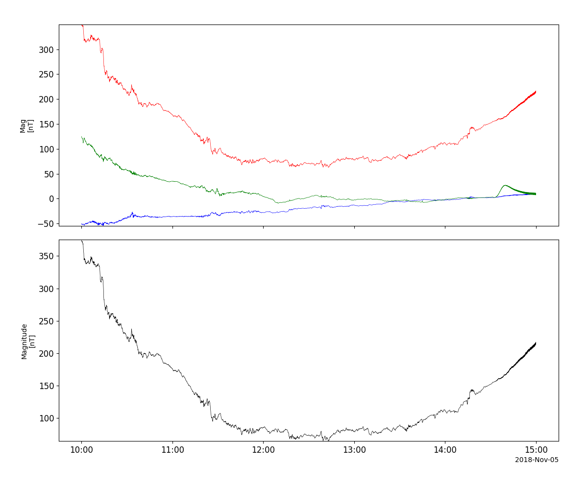
>>> emfisis_vars = pyspedas.projects.rbsp.emfisis(trange=['2018-11-5/10:00', '2018-11-5/15:00'], datatype='magnetometer', level='l3', time_clip=True)
>>> tplot(['Mag', 'Magnitude'])
Example
import pyspedas
from pyspedas import tplot
emfisis_vars = pyspedas.projects.rbsp.emfisis(trange=['2018-11-5/10:00', '2018-11-5/15:00'], datatype='magnetometer', level='l3', time_clip=True)
tplot(['Mag', 'Magnitude'])
Electric Field and Waves Suite (EFW)
- pyspedas.projects.rbsp.efw(trange=['2015-11-5', '2015-11-6'], probe='a', datatype='spec', level='l3', suffix='', prefix='', force_download=False, get_support_data=False, varformat=None, varnames=[], downloadonly=False, notplot=False, no_update=False, time_clip=False)[source]
This function loads data from the Electric Field and Waves Suite (EFW)
- Parameters:
trange (
listofstr, default[``’2015-11-5’, ``'2015-11-6']) – time range of interest [starttime, endtime] with the format ‘YYYY-MM-DD’,’YYYY-MM-DD’] or to specify more or less than a day [‘YYYY-MM-DD/hh:mm:ss’,’YYYY-MM-DD/hh:mm:ss’]probe (
strorlistofstr, default'a') – Spacecraft probe name: ‘a’ or ‘b’datatype (
str, default'spec') – Data type. Valid options are specific to different data levels.level (
str, default'l3') – Data level. Valid options: ‘l1’, ‘l2’, ‘l3’, ‘l4’prefix (
str, optional) – The tplot variable names will be given this prefix. By default, no prefix is added.suffix (
str, optional) – The tplot variable names will be given this suffix. By default, no suffix is added.force_download (
bool, defaultFalse) – Download file even if local version is more recent than server versionget_support_data (
bool, defaultFalse) – Data with an attribute “VAR_TYPE” with a value of “support_data” will be loaded into tplot. By default, only loads in data with a “VAR_TYPE” attribute of “data”.varformat (
str, optional) – The file variable formats to load into tplot. Wildcard character “*” is accepted. By default, all variables are loaded in.varnames (
listofstr, optional) – List of variable names to load (if not specified, all data variables are loaded)downloadonly (
bool, defaultFalse) – Set this flag to download the CDF files, but not load them into tplot variablesnotplot (
bool, defaultFalse) – Return the data in hash tables instead of creating tplot variablesno_update (
bool, defaultFalse) – If set, only load data from your local cachetime_clip (
bool, defaultFalse) – Time clip the variables to exactly the range specified in the trange keyword
- Returns:
tvars – List of created tplot variables or dict of data tables if notplot is True.
- Return type:
Examples
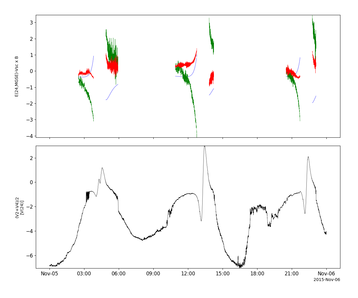
>>> efw_vars = pyspedas.projects.rbsp.efw(trange=['2015-11-5', '2015-11-6'], level='l3')
>>> tplot(['efield_in_inertial_frame_spinfit_mgse', 'spacecraft_potential'])
Example
import pyspedas
from pyspedas import tplot
efw_vars = pyspedas.projects.rbsp.efw(trange=['2015-11-5', '2015-11-6'], level='l3')
tplot(['efield_in_inertial_frame_spinfit_mgse', 'spacecraft_potential'])
Radiation Belt Storm Probes Ion Composition Experiment (RBSPICE)
- pyspedas.projects.rbsp.rbspice(trange=['2018-11-5', '2018-11-6'], probe='a', datatype='TOFxEH', level='l3', prefix='', suffix='', force_download=False, get_support_data=True, varformat=None, varnames=[], downloadonly=False, notplot=False, no_update=False, time_clip=False)[source]
This function loads data from the Radiation Belt Storm Probes Ion Composition Experiment (RBSPICE) instrument
- Parameters:
trange (
listofstr, default[``’2018-11-5’, ``'2018-11-6']) – time range of interest [starttime, endtime] with the format ‘YYYY-MM-DD’,’YYYY-MM-DD’] or to specify more or less than a day [‘YYYY-MM-DD/hh:mm:ss’,’YYYY-MM-DD/hh:mm:ss’]probe (
strorlistofstr, default'a') – Spacecraft probe name: ‘a’ or ‘b’datatype (
str, default'TOFxEH') – Data type; Valid options are specific to different data levels.level (
str, default'l3') – Data level. Valid options: ‘l1’, ‘l2’, ‘l3’prefix (
str, optional) – The tplot variable names will be given this prefix. By default, no prefix is added.suffix (
str, optional) – The tplot variable names will be given this suffix. By default, no suffix is added.force_download (
bool, defaultFalse) – Download file even if local version is more recent than server version.get_support_data (
bool, defaultTrue) – Data with an attribute “VAR_TYPE” with a value of “support_data” will be loaded into tplot. By default, only loads in data with a “VAR_TYPE” attribute of “data”.varformat (
str, optional) – The file variable formats to load into tplot. Wildcard character “*” is accepted. By default, all variables are loaded in.varnames (
listofstr) – List of variable names to load (if not specified, all data variables are loaded)downloadonly (
bool, defaultFalse) – Set this flag to download the CDF files, but not load them into tplot variablesnotplot (
bool, defaultFalse) – Return the data in hash tables instead of creating tplot variablesno_update (
bool, defaultFalse) – If set, only load data from your local cachetime_clip (
bool, defaultFalse) – Time clip the variables to exactly the range specified in the trange keyword
- Returns:
tvars – List of created tplot variables or dict of data tables if notplot is True.
- Return type:
Examples
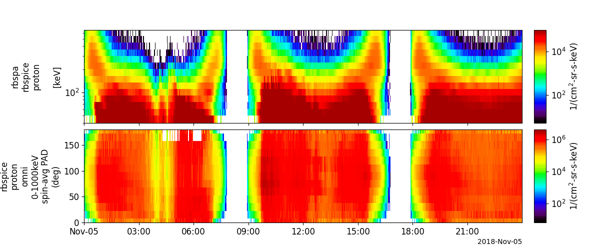
>>> rbspice_vars = pyspedas.projects.rbsp.rbspice(trange=['2018-11-5', '2018-11-6'], datatype='TOFxEH', level='l3')
>>> tplot('rbspa_rbspice_l3_TOFxEH_proton_omni_spin')
# Calculate the pitch angle distributions
>>> from pyspedas.projects.rbsp.rbspice_lib.rbsp_rbspice_pad import rbsp_rbspice_pad
>>> rbsp_rbspice_pad(probe='a', datatype='TOFxEH', level='l3')
>>> tplot('rbspa_rbspice_l3_TOFxEH_proton_omni_0-1000keV_pad_spin')
Example
import pyspedas
from pyspedas import tplot
rbspice_vars = pyspedas.projects.rbsp.rbspice(trange=['2018-11-5', '2018-11-6'], datatype='TOFxEH', level='l3')
tplot('rbspa_rbspice_l3_TOFxEH_proton_omni_spin')
# calculate the pitch angle distributions
from pyspedas.projects.rbsp.rbspice_lib.rbsp_rbspice_pad import rbsp_rbspice_pad
rbsp_rbspice_pad(probe='a', datatype='TOFxEH', level='l3')
tplot(['rbspa_rbspice_l3_TOFxEH_proton_omni_spin',
       'rbspa_rbspice_l3_TOFxEH_proton_omni_0-1000keV_pad_spin'])
- pyspedas.projects.rbsp.rbspice_lib.rbsp_rbspice_pad.rbsp_rbspice_pad(probe='a', datatype='TOFxEH', level='l3', energy=[0, 1000], bin_size=15, scopes=None)[source]
Calculate pitch angle distributions using data from the RBSP Radiation Belt Storm Probes Ion Composition Experiment (RBSPICE)
- Parameters:
probe (
strorlistofstr, default'a') – Spacecraft probe name: ‘a’ or ‘b’datatype (
str, default'TOFxEH') – desired data type: ‘TOFxEH’, ‘TOFxEnonH’level (
str, default'l3') – data level: ‘l1’,’l2’,’l3’energy (
list, default[0,1000]) – user-defined energy range to include in the calculation in keVbin_size (
float, default15) – desired size of the pitch angle bins in degreesscopes (
list, optional) – string array of telescopes to be included in PAD [0-5, default is all]
- Returns:
out – Tplot variables created
- Return type:
Examples
>>> rbspice_vars = pyspedas.projects.rbsp.rbspice(trange=['2018-11-5', '2018-11-6'], datatype='TOFxEH', level='l3')
>>> tplot('rbspa_rbspice_l3_TOFxEH_proton_omni_spin')
>>> # Calculate the pitch angle distributions
>>> from pyspedas.projects.rbsp.rbspice_lib.rbsp_rbspice_pad import rbsp_rbspice_pad
>>> rbsp_rbspice_pad(probe='a', datatype='TOFxEH', level='l3')
>>> tplot('rbspa_rbspice_l3_TOFxEH_proton_omni_0-1000keV_pad')
Calculates spin-averaged pitch angle distributions using data from the RBSP Radiation Belt Storm Probes Ion Composition Experiment (RBSPICE)
- Parameters:
probe (
strorlistofstr, default'a') – Spacecraft probe name: ‘a’ or ‘b’datatype (
str, default'TOFxEH') – desired data type: ‘TOFxEH’, ‘TOFxEnonH’level (
str, default'l3') – data level: ‘l1’,’l2’,’l3’species (
str, default'proton') – desired ion species: ‘proton’ , ‘helium’, ‘oxygen’energy (
list, default[0,1000]) – user-defined energy range to include in the calculation in keVbin_size (
float, default= 15.) – desired size of the pitch angle bins in degreesscopes (
list, optional) – string array of telescopes to be included in PAD [0-5, default is all]
- Returns:
out – Tplot variables created
- Return type:
Examples
>>> rbspice_vars = pyspedas.projects.rbsp.rbspice(trange=['2018-11-5', '2018-11-6'], datatype='TOFxEH', level='l3')
>>> tplot('rbspa_rbspice_l3_TOFxEH_proton_omni_spin')
# Calculate the pitch angle distributions
>>> from pyspedas.projects.rbsp.rbspice_lib.rbsp_rbspice_pad import rbsp_rbspice_pad_spinavg
>>> rbsp_rbspice_pad_spinavg(probe='a', datatype='TOFxEH', level='l3')
>>> tplot('rbspa_rbspice_l3_TOFxEH_proton_omni_0-1000keV_pad_spin')
Energetic Particle, Composition, and Thermal Plasma Suite (ECT) - MagEIS
- pyspedas.projects.rbsp.mageis(trange=['2015-11-5', '2015-11-6'], probe='a', datatype='', level='l3', rel='rel04', prefix='', suffix='', force_download=False, get_support_data=False, varformat=None, varnames=[], downloadonly=False, notplot=False, no_update=False, time_clip=False)[source]
This function loads data from the Energetic Particle, Composition, and Thermal Plasma Suite (ECT)
- Parameters:
trange (
listofstr, default[``’2015-11-5’, ``'2015-11-6']) – time range of interest [starttime, endtime] with the format ‘YYYY-MM-DD’,’YYYY-MM-DD’] or to specify more or less than a day [‘YYYY-MM-DD/hh:mm:ss’,’YYYY-MM-DD/hh:mm:ss’]probe (
strorlistofstr, default'a') – Spacecraft probe name: ‘a’ or ‘b’datatype (
str, default'') – Data type. Valid options are specific to different data levels.level (
str, default'l3') – Data level. Valid options: ‘l1’, ‘l2’, ‘l3’, ‘l4’rel (
str, default'rel04') – Release version of the data.prefix (
str, optional) – The tplot variable names will be given this prefix. By default, no prefix is added.suffix (
str, optional) – The tplot variable names will be given this suffix. By default, no suffix is added.force_download (
bool, defaultFalse) – Download file even if local version is more recent than server version.get_support_data (
bool, defaultFalse) – Data with an attribute “VAR_TYPE” with a value of “support_data” will be loaded into tplot. By default, only loads in data with a “VAR_TYPE” attribute of “data”.varformat (
str, optional) – The file variable formats to load into tplot. Wildcard character “*” is accepted. By default, all variables are loaded in.varnames (
listofstr, optional) – List of variable names to load (if not specified, all data variables are loaded)downloadonly (
bool, defaultFalse) – Set this flag to download the CDF files, but not load them into tplot variablesnotplot (
bool, defaultFalse) – Return the data in hash tables instead of creating tplot variablesno_update (
bool, defaultFalse) – If set, only load data from your local cachetime_clip (
bool, defaultFalse) – Time clip the variables to exactly the range specified in the trange keyword
- Returns:
tvars – List of created tplot variables or dict of data tables if notplot is True.
- Return type:
Examples
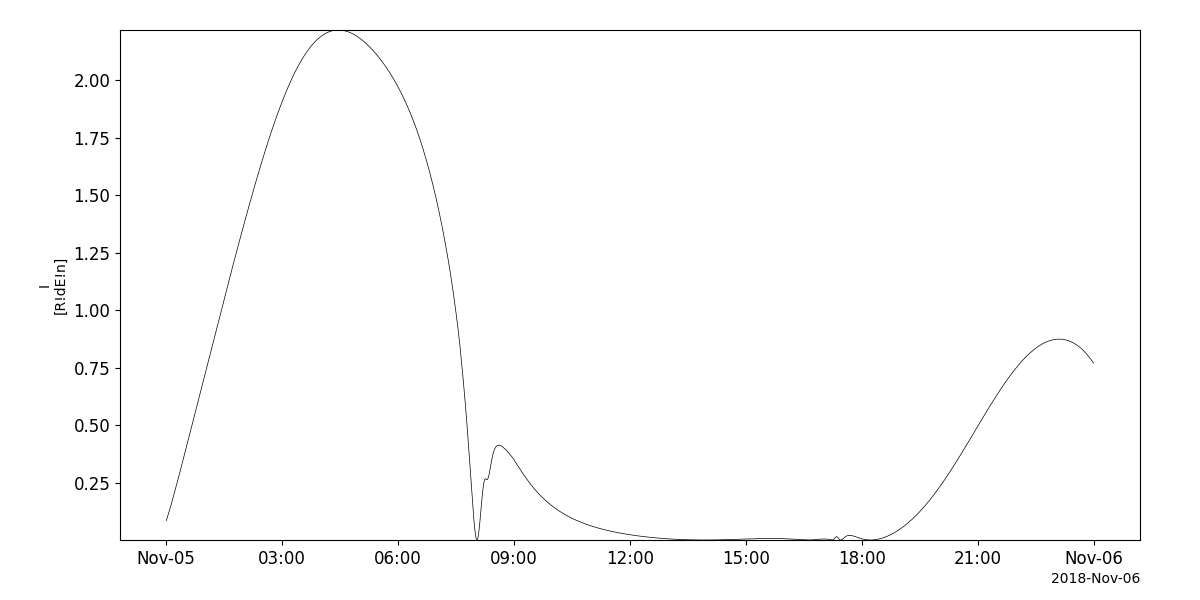
>>> mageis_vars = pyspedas.projects.rbsp.mageis(trange=['2018-11-5', '2018-11-6'], level='l3', rel='rel04')
>>> tplot('I')
Example
import pyspedas
from pyspedas import tplot
mageis_vars = pyspedas.projects.rbsp.mageis(trange=['2018-11-5', '2018-11-6'], level='l3', rel='rel04')
tplot('I')
Energetic Particle, Composition, and Thermal Plasma Suite (ECT) - HOPE
- pyspedas.projects.rbsp.hope(trange=['2015-11-5', '2015-11-6'], probe='a', datatype='moments', level='l3', rel='rel04', prefix='', suffix='', force_download=False, get_support_data=False, varformat=None, varnames=[], downloadonly=False, notplot=False, no_update=False, time_clip=False)[source]
This function loads data from the Energetic Particle, Composition, and Thermal Plasma Suite (ECT)
- Parameters:
trange (
listofstr, default[``’2015-11-5’, ``'2015-11-6']) – time range of interest [starttime, endtime] with the format ‘YYYY-MM-DD’,’YYYY-MM-DD’] or to specify more or less than a day [‘YYYY-MM-DD/hh:mm:ss’,’YYYY-MM-DD/hh:mm:ss’]probe (
strorlistofstr, default'a') – Spacecraft probe name: ‘a’ or ‘b’datatype (
str, default'moments') – Data type. Valid options are specific to different data levels.level (
str, default'l3') – Data level. Valid options: ‘l1’, ‘l2’, ‘l3’, ‘l4’rel (
str, default'rel04') – Release version of the data.prefix (
str, optional) – The tplot variable names will be given this prefix. By default, no prefix is added.suffix (
str, optional) – The tplot variable names will be given this suffix. By default, no suffix is added.force_download (
bool, defaultFalse) – Download file even if local version is more recent than server version.get_support_data (
bool, defaultFalse) – Data with an attribute “VAR_TYPE” with a value of “support_data” will be loaded into tplot. By default, only loads in data with a “VAR_TYPE” attribute of “data”.varformat (
str, optional) – The file variable formats to load into tplot. Wildcard character “*” is accepted. By default, all variables are loaded in.varnames (
listofstr, optional) – List of variable names to load (if not specified, all data variables are loaded)downloadonly (
bool, defaultFalse) – Set this flag to download the CDF files, but not load them into tplot variablesnotplot (
bool, defaultFalse) – Return the data in hash tables instead of creating tplot variablesno_update (
bool, defaultFalse) – If set, only load data from your local cachetime_clip (
bool, defaultFalse) – Time clip the variables to exactly the range specified in the trange keyword
- Returns:
tvars – List of created tplot variables or dict of data tables if notplot is True.
- Return type:
Examples
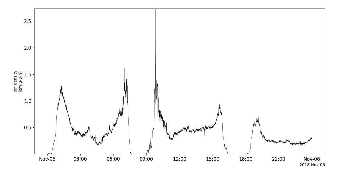
>>> hope_vars = pyspedas.projects.rbsp.hope(trange=['2018-11-5', '2018-11-6'], datatype='moments', level='l3', rel='rel04')
>>> tplot('Ion_density')
Example
import pyspedas
from pyspedas import tplot
hope_vars = pyspedas.projects.rbsp.hope(trange=['2018-11-5', '2018-11-6'], datatype='moments', level='l3', rel='rel04')
tplot('Ion_density')
Energetic Particle, Composition, and Thermal Plasma Suite (ECT) - REPT
- pyspedas.projects.rbsp.rept(trange=['2015-11-5', '2015-11-6'], probe='a', datatype='', level='l3', rel='rel03', prefix='', suffix='', force_download=False, get_support_data=False, varformat=None, varnames=[], downloadonly=False, notplot=False, no_update=False, time_clip=False)[source]
This function loads data from the Energetic Particle, Composition, and Thermal Plasma Suite (ECT)
- Parameters:
trange (
listofstr, default[``’2015-11-5’, ``'2015-11-6']) – time range of interest [starttime, endtime] with the format ‘YYYY-MM-DD’,’YYYY-MM-DD’] or to specify more or less than a day [‘YYYY-MM-DD/hh:mm:ss’,’YYYY-MM-DD/hh:mm:ss’]probe (
strorlistofstr, default'a') – Spacecraft probe name: ‘a’ or ‘b’datatype (
str, default'') – Data type. Valid options are specific to different data levels.level (
str, default'l3') – Data level. Valid options: ‘l1’, ‘l2’, ‘l3’, ‘l4’rel (
str, default'rel03') – Release version of the data.prefix (
str, optional) – The tplot variable names will be given this prefix. By default, no prefix is added.suffix (
str, optional) – The tplot variable names will be given this suffix. By default, no suffix is added.force_download (
bool, defaultFalse) – Download file even if local version is more recent than server version.get_support_data (
bool, defaultFalse) – Data with an attribute “VAR_TYPE” with a value of “support_data” will be loaded into tplot. By default, only loads in data with a “VAR_TYPE” attribute of “data”.varformat (
str, optional) – The file variable formats to load into tplot. Wildcard character “*” is accepted. By default, all variables are loaded in.varnames (
listofstr, optional) – List of variable names to load (if not specified, all data variables are loaded)downloadonly (
bool, defaultFalse) – Set this flag to download the CDF files, but not load them into tplot variablesnotplot (
bool, defaultFalse) – Return the data in hash tables instead of creating tplot variablesno_update (
bool, defaultFalse) – If set, only load data from your local cachetime_clip (
bool, defaultFalse) – Time clip the variables to exactly the range specified in the trange keyword
- Returns:
tvars – List of created tplot variables or dict of data tables if notplot is True.
- Return type:
Examples
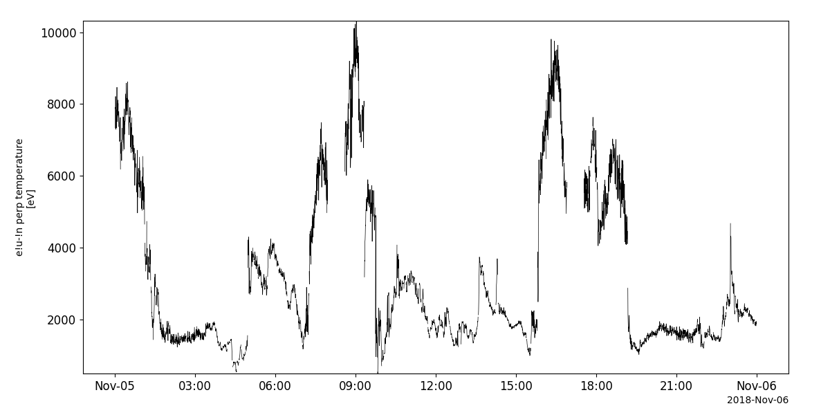
>>> rept_vars = pyspedas.projects.rbsp.rept(trange=['2018-11-5', '2018-11-6'], level='l3', rel='rel03')
>>> tplot('FEDU')
Example
import pyspedas
from pyspedas import tplot
rept_vars = pyspedas.projects.rbsp.rept(trange=['2018-11-5', '2018-11-6'], level='l3', rel='rel03')
tplot('Tperp_e_200')
Relativistic Proton Spectrometer (RPS)
- pyspedas.projects.rbsp.rps(trange=['2015-11-5', '2015-11-6'], probe='a', datatype='rps-1min', level='l2', prefix='', suffix='', force_download=False, get_support_data=True, varformat=None, varnames=[], downloadonly=False, notplot=False, no_update=False, time_clip=False)[source]
This function loads data from the Relativistic Proton Spectrometer (RPS)
- Parameters:
trange (
listofstr, default[``’2015-11-5’, ``'2015-11-6']) – time range of interest [starttime, endtime] with the format ‘YYYY-MM-DD’,’YYYY-MM-DD’] or to specify more or less than a day [‘YYYY-MM-DD/hh:mm:ss’,’YYYY-MM-DD/hh:mm:ss’]probe (
strorlistofstr, default'a') – Spacecraft probe name: ‘a’ or ‘b’datatype (
str, default'rps-1min') – Data type. Valid options are specific to different data levels.level (
str, default'l2') – Data level. Valid options: ‘l1’, ‘l2’, ‘l3’, ‘l4’prefix (
str, optional) – The tplot variable names will be given this prefix. By default, no prefix is added.suffix (
str, optional) – The tplot variable names will be given this suffix. By default, no suffix is added.force_download (
bool, defaultFalse) – Download file even if local version is more recent than server version.get_support_data (
bool, defaultTrue) – Data with an attribute “VAR_TYPE” with a value of “support_data” will be loaded into tplot. By default, only loads in data with a “VAR_TYPE” attribute of “data”.varformat (
str, optional) – The file variable formats to load into tplot. Wildcard character “*” is accepted. By default, all variables are loaded in.varnames (
listofstr, optional) – List of variable names to load (if not specified, all data variables are loaded)downloadonly (
bool, defaultFalse) – Set this flag to download the CDF files, but not load them into tplot variablesnotplot (
bool, defaultFalse) – Return the data in hash tables instead of creating tplot variablesno_update (
bool, defaultFalse) – If set, only load data from your local cachetime_clip (
bool, defaultFalse) – Time clip the variables to exactly the range specified in the trange keyword
- Returns:
tvars – List of created tplot variables or dict of data tables if notplot is True.
- Return type:
Examples
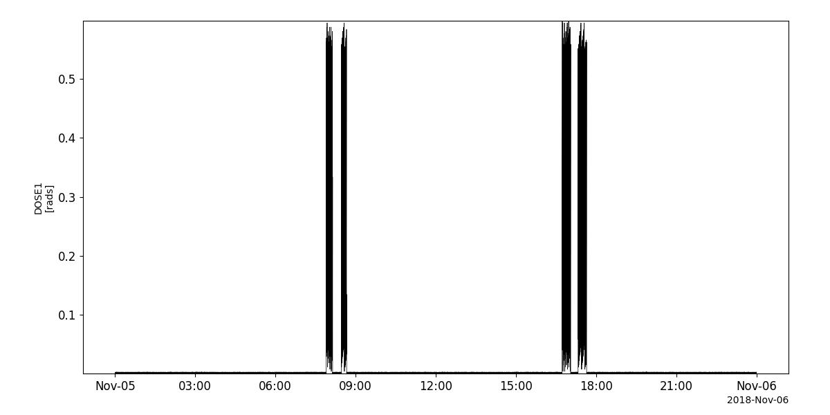
>>> rps_vars = pyspedas.projects.rbsp.rps(trange=['2018-11-5', '2018-11-6'], datatype='rps', level='l2')
>>> tplot('DOSE1')
Example
import pyspedas
from pyspedas import tplot
rps_vars = pyspedas.projects.rbsp.rps(trange=['2018-11-5', '2018-11-6'], datatype='rps', level='l2')
tplot('DOSE1')