NOFS)

The routines in this module can be used to load data from the Communications/Navigation Outage Forecasting System (C/NOFS) mission.

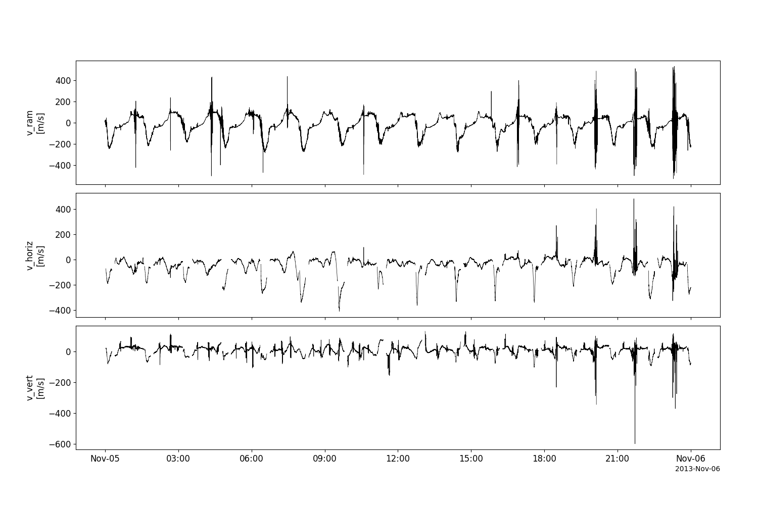
Coupled Ion-Neutral Dynamics Investigation (CINDI)

pyspedas.cnofs.cindi(trange=['2013-11-5', '2013-11-6'], suffix='', get_support_data=False, varformat=None, varnames=[], downloadonly=False, notplot=False, no_update=False, time_clip=False)[source]

This function loads data from the Coupled Ion-Neutral Dynamics Investigation (CINDI)

Parameters:

trange (list of str) – time range of interest [starttime, endtime] with the format ‘YYYY-MM-DD’,’YYYY-MM-DD’] or to specify more or less than a day [‘YYYY-MM-DD/hh:mm:ss’,’YYYY-MM-DD/hh:mm:ss’] Default: [‘2013-11-5’, ‘2013-11-6’]
suffix (str) – The tplot variable names will be given this suffix. By default, no suffix is added.
get_support_data (bool) – Data with an attribute “VAR_TYPE” with a value of “support_data” will be loaded into tplot. By default, only loads in data with a “VAR_TYPE” attribute of “data”.
varformat (str) – The file variable formats to load into tplot. Wildcard character “*” is accepted. By default, all variables are loaded in.
varnames (list of str) – List of variable names to load (if not specified, all data variables are loaded)
downloadonly (bool) – Set this flag to download the CDF files, but not load them into tplot variables Default: False
notplot (bool) – Return the data in hash tables instead of creating tplot variables Default: False
no_update (bool) – If set, only load data from your local cache Default: False
time_clip (bool) – Time clip the variables to exactly the range specified in the trange keyword Default: False

Return type:

List of tplot variables created.

Example:

>>> import pyspdedas
>>> from pytplot import tplot
>>> cindi_vars = pyspedas.cnofs.cindi(trange=['2013-11-5', '2013-11-6'])
>>> tplot(['ionVelocityX', 'ionVelocityY', 'ionVelocityZ'])

Example

import pyspedas
from pytplot import tplot
cindi_vars = pyspedas.cnofs.cindi(trange=['2013-11-5', '2013-11-6'])
tplot(['ionVelocityX', 'ionVelocityY', 'ionVelocityZ'])

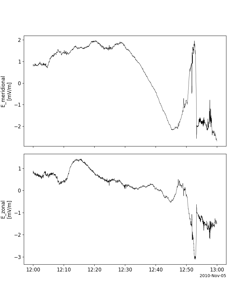
Vector Electric Field Instrument (VEFI)

pyspedas.cnofs.vefi(trange=['2010-11-5', '2010-11-6'], datatype='efield_1sec', suffix='', get_support_data=False, varformat=None, varnames=[], downloadonly=False, notplot=False, no_update=False, time_clip=False)[source]

This function loads data from the Vector Electric Field Instrument (VEFI)

Parameters:

trange (list of str) – time range of interest [starttime, endtime] with the format ‘YYYY-MM-DD’,’YYYY-MM-DD’] or to specify more or less than a day [‘YYYY-MM-DD/hh:mm:ss’,’YYYY-MM-DD/hh:mm:ss’] Default: [‘2010-11-5’, ‘2010-11-6’]
datatype (str) – String specifying datatype (options: ‘efield_1sec’, ‘bfield_1sec’, ‘ld_500msec’) Default: ‘efield_1sec’
suffix (str) – The tplot variable names will be given this suffix. Default: ‘’, no suffix is added.
get_support_data (bool) – Data with an attribute “VAR_TYPE” with a value of “support_data” will be loaded into tplot. Default: False. Only loads in data with a “VAR_TYPE” attribute of “data”.
varformat (str) – The file variable formats to load into tplot. Wildcard character “*” is accepted. Default: None. All variables are loaded in.
varnames (list of str) – List of variable names to load Default: []. If not specified, all data variables are loaded
downloadonly (bool) – Set this flag to download the CDF files, but not load them into tplot variables Default: False
notplot (bool) – Return the data in hash tables instead of creating tplot variables Default: False
no_update (bool) – If set, only load data from your local cache Default: False
time_clip (bool) – Time clip the variables to exactly the range specified in the trange keyword Default: False

Return type:

List of tplot variables created.

Example:

>>> import pyspdedas
>>> from pytplot import tplot
>>> vefi_vars = pyspedas.cnofs.vefi(trange=['2013-11-5', '2013-11-6'])
>>> tplot(['E_meridional', 'E_zonal'])

Example

import pyspedas
from pytplot import tplot
vefi_vars = pyspedas.cnofs.vefi(trange=['2010-11-5/12:00', '2010-11-5/13:00'])
tplot(['E_meridional', 'E_zonal'])

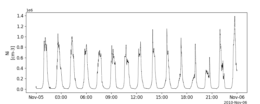
Planar Langmuir Probe (PLP)

pyspedas.cnofs.plp(trange=['2013-11-5', '2013-11-6'], suffix='', get_support_data=False, varformat=None, varnames=[], downloadonly=False, notplot=False, no_update=False, time_clip=False)[source]

This function loads data from the Planar Langmuir Probe (PLP)

Parameters:

trange (list of str) – time range of interest [starttime, endtime] with the format ‘YYYY-MM-DD’,’YYYY-MM-DD’] or to specify more or less than a day [‘YYYY-MM-DD/hh:mm:ss’,’YYYY-MM-DD/hh:mm:ss’] Default: [‘2013-11-5’, ‘2013-11-6’]
suffix (str) – The tplot variable names will be given this suffix. Default: ‘’, no suffix is added.
get_support_data (bool) – Data with an attribute “VAR_TYPE” with a value of “support_data” will be loaded into tplot. Default: False. Only loads in data with a “VAR_TYPE” attribute of “data”.
varformat (str) – The file variable formats to load into tplot. Wildcard character “*” is accepted. Default: None. All variables are loaded in.
varnames (list of str) – List of variable names to load. Default: []. If not specified, all data variables are loaded
downloadonly (bool) – Set this flag to download the CDF files, but not load them into tplot variables. Default: False
notplot (bool) – Return the data in hash tables instead of creating tplot variables. Default: False
no_update (bool) – If set, only load data from your local cache. Default: False
time_clip (bool) – Time clip the variables to exactly the range specified in the trange keyword. Default: False

Return type:

List of tplot variables created.

Example:

>>> import pyspdedas
>>> from pytplot import tplot
>>> plp_vars = pyspedas.cnofs.plp(trange=['2010-11-5', '2010-11-6'])
>>> tplot('Ni')

Example

import pyspedas
from pytplot import tplot
plp_vars = pyspedas.cnofs.plp(trange=['2010-11-5', '2010-11-6'])
tplot('Ni')