Swarm
The routines in this module can be used to load data from the Swarm mission.
Vector Field Magnetometer (VFM)
- pyspedas.projects.swarm.mag(trange=['2017-03-27/06:00', '2017-03-27/08:00'], probe='a', datatype='hr', level='l1b', prefix='', suffix='', varnames=[], time_clip=False, force_download=False)[source]
Loads data from the Vector Field Magnetometer (VFM).
- Parameters:
trange (
listofstr, default[``’2017-03-27/06:00’, ``'2017-03-27/08:00']) – Time range of interest [starttime, endtime] with the format ‘YYYY-MM-DD’ or ‘YYYY-MM-DD/hh:mm:ss’.probe (
strorlistofstr, default'a') – Swarm spacecraft ID (‘a’, ‘b’, and/or ‘c’).datatype (
str, default'hr') – Data type; valid options: ‘hr’ (high resolution), ‘lr’ (low resolution).level (
str, default'l1b') – Data level; options: ‘l1b’.prefix (
str, optional) – The tplot variable names will be given this prefix. By default, no prefix is added.suffix (
str, optional) – The tplot variable names will be given this suffix. By default, no suffix is added.varnames (
listofstr, optional) – List of variable names to load. If not specified, all data variables are loaded.time_clip (
bool, defaultFalse) – Time clip the variables to exactly the range specified in the trange keyword.force_download (
bool, defaultFalse) – Swarm data is requested via HAPI. This parameter always ignored and reserved for compatibility.
- Returns:
out_vars – List of tplot variables created.
- Return type:
Examples
To load and plot Magnetometer (MAG) data from the Swarm mission for probe ‘c’ over a specific time range, you can use the following commands:
>>> import pyspedas
>>> from pyspedas import tplot
# Load MAG data for probe ‘c’ >>> mag_vars = pyspedas.projects.swarm.mag(probe=’c’, trange=[‘2017-03-27/06:00’, ‘2017-03-27/08:00’], datatype=’hr’)
# Plot the loaded MAG data >>> tplot(‘swarmc_B_VFM’)
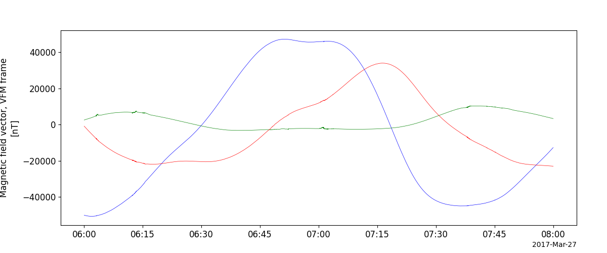
Example
import pyspedas
from pyspedas import tplot
mag_vars = pyspedas.projects.swarm.mag(probe='c', trange=['2017-03-27/06:00', '2017-03-27/08:00'], datatype='hr')
tplot('swarmc_B_VFM')