Magnetic Field Models

This module provides a set of routines that can be used to calculate various magnetic field models, using Sheng Tian’s implementation of the geopack library (https://github.com/tsssss/geopack).

The routines documented here each accept an input tplot variable, specifying the times and positions at which the field models are to be evaluated. If units and coordinate system metadata are present, it will be used to convert internally to GSM coordinates and units of Re (earth radii). Missing or incorrect metadata can be provided or overridden via the coord_in and units_in keyword arguments.

Each field model has its own set of parameters. The parameters may be passed as tplot variables names, in which case they are interpolated to the times specified in the input position variable. If a scalar value is passed, it is used for all input times. If an n-element array is passed. n is expected to match the number of input times/positions, and the n-th array element will be used as the parameter value for the n-th model evaluation.

Most of these routines also accept a boolean ‘autoload’ parameter. If True, any provided model parameters will be ignored, and the parameters will be derived from data loaded from various data sources: Kyoto WDC for Kp/iopt values, OMNIweb for solar wind parameters, or directly from K. Tysganenko’s web site for certain models and parameters.

The modeled B vectors are returned as tplot variables in units of nT. By default, they will be returned in the GSM coordinate system, but this can be changed via the coord_out keyword parameter.

Managing model parameters

As mentioned above, most of the field modeling and tracing routines support a boolean ‘autoload’ parameter, which will load the relevant solar wind and magnetospheric parameters from OMNIweb, the Kyoto WDC, or other sources.

However, sometimes it is necessary or desirable to obtain or synthesize these parameters from other data. The routines describe here allow arbitrary constants, tplot variables, or data arrays to be passed to the modeling and tracing routines, with appropriate interpolation and sanitization performed automatically.

Parameters to each model can be supplied as tplot variables (to be interpolated to the input times), scalars (to be applied to all times), as arrays (length equal to number of input times), or as 10-element or n-by-10 element ‘parmod’ arrays (all model parameters passed in a single array).

The clean_model_parameters routine takes a single model parameter and performs the necessary NaN-stripping, replication, or interpolation to return a properly sized array matching the input data.

pyspedas.geopack.clean_model_parameters(input_times, model_param, method='linear') → ndarray[source]

Create a 1D array of model parameter values from a scalar, array, or tplot variable name.

Parameters:

input_times (ndarray of floats) – The timestamp array of the input tplot variable. Model parameters will be interpolated to these times.
model_param (Any) – A scalar floating point value, array of values, or tplot variable name. Scalars are repeated to match the number of input timestamps. Arrays are taken as-is, after checking that the array size matches the number of timestamps. tplot variables are interpolated to input_times after removing NaN values.
method (str) – The interpolation method to use. Kp and iopt values are not from a continuous scale, so they should be interpolated with method=”nearest”. Default: “linear”

Returns:

An array of cleaned parameter values, with the same number of elements as the input times.

Return type:

ndarray of floats

pyspedas.get_t89_parameters(pos_var, kp, iopt, parmod, autoload, igrf_only)[source]

Construct an array of T89 model parameters from individual scalar values, arrays, or tplot variables.

Parameters:

pos_var (str) – Input times and positions to be used
kp (Any) – The Kp parameter to use for the t89 model (scalar, array, or tplot variable name)
iopt (Any) – The model parameter to use for the t89 model (scalar, array, or tplot variable name)
igrf_only (bool) – For the t89 model, if true, only include the IGRF standard field.
parmod (Any) – A 10-element or n-by-10 array of parameter values (or an equivalent tplot variable) to be replicated or used as-is for model parameters
autoload (bool) – If True, ignore any passed parameters and download model parameters from an appropriate source.

Returns:

An n by 10, cleaned array of floating point parameters interpolated or replicated to the input timestamps

Return type:

ndarray of floats

pyspedas.get_t96_parameters(pos_var, pdyn, dst, byimf, bzimf, parmod, autoload)[source]

Construct an array of T96 model parameters from individual scalar values, arrays, or tplot variables.

Parameters:

pos_var (str) – Input times and positions to be used
pdyn (Any) – Solar wind dynamic pressure in nPa
dst (Any) – Dst index in nT
byimf (Any) – Y component of interplanetary magnetic field
bzimf (Any) – Z component of interplanetary magnetic field
parmod (ndarray) – A 10-element or n-by-10 array of parameter values to be replicated or used as-is for model parameters
autoload (bool) – If True, ignore any passed parameters and download model parameters from an appropriate source.

Returns:

An n by 10, cleaned array of floating point parameters interpolated or replicated to the input timestamps

Return type:

ndarray of floats

pyspedas.get_t01_parameters(pos_var, pdyn=None, dst=None, byimf=None, bzimf=None, g1=None, g2=None, parmod=None, autoload=False)[source]

Construct an array of T01 model parameters from individual scalar values, arrays, or tplot variables.

Parameters:

pos_var (str) – Input times and positions to be used
pdyn (Any) – Solar wind dynamic pressure in nPa
dst (Any) – Dst index in nT
byimf (Any) – Y component of interplanetary magnetic field
bzimf (Any) – Z component of interplanetary magnetic field
g1 (Any) – g1 index value
g2 (Any) – g2 index value
parmod (Any) – A 10-element or n-by-10 array of parameter values (or equivalent tplot variable) to be replicated or used as-is for model parameters
autoload (bool) – If True, ignore any passed parameters and download model parameters from an appropriate source.

Returns:

An n by 10, cleaned array of floating point parameters interpolated or replicated to the input timestamps

Return type:

ndarray of floats

pyspedas.get_ts04_parameters(pos_var, pdyn, dst, byimf, bzimf, w1, w2, w3, w4, w5, w6, parmod, autoload)[source]

Construct an array of TS04 model parameters from individual scalar values, arrays, or tplot variables.

Parameters:

pos_var (str) – Input times and positions to be used
pdyn (Any) – Solar wind dynamic pressure in nPa
dst (Any) – Dst index in nT
byimf (Any) – Y component of interplanetary magnetic field
bzimf (Any) – Z component of interplanetary magnetic field
w1 (Any) – w1 index value
w2 (Any) – w2 index value
w3 (Any) – w3 index value
w4 (Any) – w4 index value
w5 (Any) – w5 index value
w6 (Any) – w6 index value
parmod (ndarray) – A 10-element or n-by-10 array of parameter values to be replicated or used as-is for model parameters
autoload (bool) – If True, ignore any passed parameters and download model parameters from an appropriate source.

Returns:

An n by 10, cleaned array of floating point parameters interpolated or replicated to the input timestamps

Return type:

ndarray of floats

IDL SPEDAS compatibility: get_tsy_params

Note: This routine is provided as a convenience for users wishing to port IDL SPEDAS field line tracing code to PySPEDAS. In most cases, passing ‘autoload=True’ to the modeling or field line tracing routines, or using one of the model-specific routines described above will be the easiest and cleanest way to prepare the model parameters.

To generate the “parmod” variable using Dst and solar wind data, use the get_tsy_params routine.

pyspedas.get_tsy_params(dst_tvar, imf_tvar, Np_tvar, Vp_tvar, model, pressure_tvar=None, newname=None, speed=False, g_variables=None)[source]

This procedure will interpolate inputs, generate Tsyganenko model parameters and store them in a tplot variable that can be passed directly to the model procedure.

Input

dst_tvar: str
tplot variable containing the Dst index

imf_tvar: str
tplot variable containing the interplanetary magnetic field vector in GSM coordinates

Np_tvar: str
tplot variable containing the solar wind ion density (cm**-3)

Vp_tvar: str
tplot variable containing the proton velocity

model: str
Tsyganenko model; should be: ‘T89’, T96’, ‘T01’,’TS04’

Parameters:

newname (str) – name of the output variable; default: t96_par, ‘t01_par’ or ‘ts04_par’, depending on the model
speed (bool) – Flag to indicate Vp_tvar is speed, and not velocity (defaults to False)
pressure_tvar (str) – Set this to specify a tplot variable containing solar wind dynamic pressure data. If not supplied, it will be calculated internally from proton density and proton speed.

returns:

Name of the tplot variable containing the parameters.

rtype:

str

Notes

The parameters are:

(1) solar wind pressure pdyn (nanopascals),
(2) dst (nanotesla),
(3) byimf,
(4) bzimf (nanotesla)
(5-10) indices w1 - w6, calculated as time integrals from the beginning of a storm

get_tsy_params Example

# load Dst and solar wind data
import pyspedas
pyspedas.projects.kyoto.dst(trange=['2015-10-16', '2015-10-17'])
pyspedas.projects.omni.data(trange=['2015-10-16', '2015-10-17'])

# join the components of B into a single variable
# BX isn't used
from pyspedas import join_vec
join_vec(['BX_GSE', 'BY_GSM', 'BZ_GSM'])

from pyspedas.get_tsy_params import get_tsy_params
params = get_tsy_params('kyoto_dst',
                     'BX_GSE-BY_GSM-BZ_GSM_joined',
                     'proton_density',
                     'flow_speed',
                     't96', # or 't01', 'ts04'
                     pressure_tvar='Pressure',
                     speed=True)

IGRF (IGRF)

This is the underlying basic field model. The rest of the Geopack models are implemented as small corrections to be added to the IGRF field.

pyspedas.tigrf(pos_var, units_in: str = None, coord_in: str = None, coord_out: str = 'GSM', suffix='')[source]

tplot wrapper for the functional interface to Sheng Tian’s implementation of the Tsyganenko T89 and IGRF model:

https://github.com/tsssss/geopack

Parameters:

pos_var (str) – tplot variable containing the position data.
coord_in (str) – (Optional) Coordinate system of input variable, overrides any metadata in pos_var. Must be convertible to GSM.
units_in (str) – (Optional) Units of input variable, overrides any metadata in pos_var. Valid options: [‘km’, ‘Re’]
coord_out (str) – (Optional) Coordinate system of output variable. Must be convertible from GSM. Default: ‘GSM’
suffix (str) – Suffix to append to the tplot output variable

Returns:

Name of the tplot variable containing the model data

Return type:

str

Tsyganenko 89 (T89)

pyspedas.tt89(pos_var, units_in: str = None, coord_in: str = None, kp=None, iopt=None, parmod=None, autoload=False, coord_out: str = 'GSM', suffix: str = '', igrf_only=False)[source]

Evaluate the T89 field model at the times/positions specified by an input tplot variable.

Parameters:

pos_var (str) – tplot variable containing the position data.
coord_in (str) – (Optional) Coordinate system of input variable, overrides any metadata in pos_var. Must be convertible to GSM.
units_in (str) – (Optional) Units of input variable, overrides any metadata in pos_var. Valid options: [‘km’, ‘Re’]

iopt (str | int (Optional)) – If present, specifies the ground disturbance level. If iopt is a string, it is interpreted as a tplot variable name and interpolated to the times in pos_gsm_tvar. iopt is related to the Kp index:

=========  ======== =======  =======  =======  =======  =======
iopt= 1       2        3        4        5        6      7
kp=  0,0+  1-,1,1+  2-,2,2+  3-,3,3+  4-,4,4+  5-,5,5+  >= 6-
=========  ======== =======  =======  =======  =======  =======

kp (str | float (Optional)) – If present, specifies the Kp index, which will be converted to the equivalent iopt value. If kp is a string, it is interpreted as a tplot variable name and interpolated to the times in pos_gsm_tvar.
parmod (str | array[float] (Optional)) – If present, specifies an n by 10 elements floating point array of parameters. The first element is interpreted as the iopt value, and the rest are ignored. If parmod is a string, it is interpreted as a tplot variable name and interpolated to the times in pos_gsm_tvar.
autoload (boolean (Optional)) – If True, ignore any other parameters provided, load Kp index data from the Kyoto WDC, and convert to iopt values.
coord_out (str) – (Optional) Coordinate system of output variable. Must be convertible from GSM. Default: ‘GSM’
suffix (str (Optional)) – Suffix to append to the tplot output variable
igrf_only (bool) – If True, only return the IGRF field, without adding the T89 correction. This usage is deprecated…please use the tigrf() routine if that’s what you need. Default: False

Returns:

Name of the tplot variable containing the model data

Return type:

str

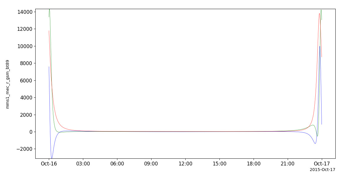
T89 Example

# load some spacecraft position data
import pyspedas
pyspedas.projects.mms.mec(trange=['2015-10-16', '2015-10-17'])

# calculate the field using the T89 model
from pyspedas.geopack import tt89
tt89('mms1_mec_r_gsm')

from pyspedas import tplot
tplot('mms1_mec_r_gsm_bt89')

Tsyganenko 96 (T96)

pyspedas.tt96(pos_var, units_in: str = None, coord_in: str = None, pdyn=None, dst=None, byimf=None, bzimf=None, parmod=None, autoload=False, coord_out: str = 'GSM', suffix='')[source]

Evaluate the T96 field model at the times and positions specified by an input tplot variable.

This is a tplot wrapper for the functional interface to Sheng Tian’s implementation of the Tsyganenko 96 and IGRF model:

https://github.com/tsssss/geopack

Parameters:

pos_var (str) – tplot variable containing the position data (km) in GSM coordinates
coord_in (str) – (Optional) Coordinate system of input variable, overrides any metadata in pos_var. Must be convertible to GSM.
units_in (str) – (Optional) Units of input variable, overrides any metadata in pos_var. Valid options: [‘km’, ‘Re’]
parmod (str) – A tplot variable containing a 10-element model parameter array (vs. time). The timestamps should match the timestamps in the input position variable. Only the first 4 elements are used:
```
(1) solar wind pressure pdyn (nanopascals)
(2) dst (nanotesla)
(3) byimf (nanotesla)
(4) bzimf (nanotesla)
```
coord_out (str) – (Optional) Coordinate system of output variable. Must be convertible from GSM. Default: ‘GSM’
suffix (str) – Suffix to append to the tplot output variable

Returns:

Name of the tplot variable containing the model data

Return type:

str

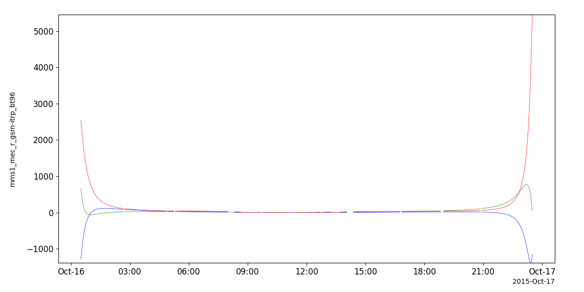
T96 Example

# load some spacecraft position data
import pyspedas
pyspedas.projects.mms.mec(trange=['2015-10-16', '2015-10-17'])

# calculate the params using the solar wind data; see the "Solar Wind Parameters" section below for an example

# interpolate the MEC timestamps to the solar wind timestamps
from pyspedas import tinterpol
tinterpol('mms1_mec_r_gsm', 'proton_density')

# calculate the field using the T96 model
from pyspedas.geopack import tt96
tt96('mms1_mec_r_gsm-itrp', parmod=params)

from pyspedas import tplot
tplot('mms1_mec_r_gsm-itrp_bt96')

Tsyganenko 2001 (T01)

pyspedas.tt01(pos_var, units_in: str = None, coord_in: str = None, pdyn=None, dst=None, byimf=None, bzimf=None, g1=None, g2=None, parmod=None, coord_out: str = 'GSM', suffix='', autoload=False)[source]

Evaluate the T01 field model at the times and positions specified by an input tplot variable.

This is a tplot wrapper for the functional interface to Sheng Tian’s implementation of the Tsyganenko 2001 and IGRF model:

https://github.com/tsssss/geopack

Parameters:

pos_var (str) – tplot variable containing the position data.
coord_in (str) – (Optional) Coordinate system of input variable, overrides any metadata in pos_var. Must be convertible to GSM.
units_in (str) – (Optional) Units of input variable, overrides any metadata in pos_var. Valid options: [‘km’, ‘Re’]

parmod (string) – A tplot variable containing a 10-element model parameter array (vs. time). The timestamps should match the input position variable. Only the first 6 elements are used:

(1) solar wind pressure pdyn (nanopascals),
(2) dst (nanotesla)
(3) byimf (nanotesla)
(4) bzimf (nanotesla)
(5) g1-index
(6) g2-index  (see Tsyganenko [2001] for an exact definition of these two indices)

suffix (str) – Suffix to append to the tplot output variable

Returns:

Name of the tplot variable containing the model data

Return type:

str

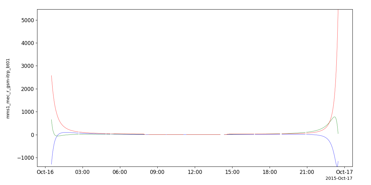
T01 Example

# load some spacecraft position data
import pyspedas
pyspedas.projects.mms.mec(trange=['2015-10-16', '2015-10-17'])

# calculate the params using the solar wind data; see the "Solar Wind Parameters" section below for an example

# interpolate the MEC timestamps to the solar wind timestamps
from pyspedas import tinterpol
tinterpol('mms1_mec_r_gsm', 'proton_density')

# calculate the field using the T01 model
from pyspedas.geopack import tt01
tt01('mms1_mec_r_gsm-itrp', parmod=params)

from pyspedas import tplot
tplot('mms1_mec_r_gsm-itrp_bt01')

Tsyganenko-Sitnov 2004 (TS04)

pyspedas.tts04(pos_var, units_in: str = None, coord_in: str = None, pdyn=None, dst=None, byimf=None, bzimf=None, w1=None, w2=None, w3=None, w4=None, w5=None, w6=None, autoload=False, parmod=None, coord_out: str = 'GSM', suffix='')[source]

Evaluate the TS04 field model at the times and locations specified by an input tplot variable.

This is a tplot wrapper for the functional interface to Sheng Tian’s implementation of the Tsyganenko-Sitnov (2004) storm-time geomagnetic field model

https://github.com/tsssss/geopack

Input

pos_var: str
tplot variable containing the position data (km) in GSM coordinates

Parameters:

pos_var (str) – tplot variable containing the position data.
coord_in (str) – (Optional) Coordinate system of input variable, overrides any metadata in pos_var. Must be convertible to GSM.
units_in (str) – (Optional) Units of input variable, overrides any metadata in pos_var. Valid options: [‘km’, ‘Re’]

parmod (str) – A tplot variable containing the model parameters as a 10-element array (vs. time). The timestamps should match the times in the input position variable. The motdl:

(1) solar wind pressure pdyn (nanopascals),
(2) dst (nanotesla),
(3) byimf,
(4) bzimf (nanotesla)
(5-10) indices w1 - w6, calculated as time integrals from the beginning of a storm

coord_out (str) – (Optional) Coordinate system of output variable. Must be convertible from GSM. Default: ‘GSM’
suffix (str) – Suffix to append to the tplot output variable

returns:

Name of the tplot variable containing the model data

rtype:

str

TS04 Example

# load some spacecraft position data
import pyspedas
pyspedas.projects.mms.mec(trange=['2015-10-16', '2015-10-17'])

# calculate the params using the solar wind data; see the "Solar Wind Parameters" section below for an example

# interpolate the MEC timestamps to the solar wind timestamps
from pyspedas import tinterpol
tinterpol('mms1_mec_r_gsm', 'proton_density')

# calculate the field using the TS04 model
from pyspedas.geopack import tts04
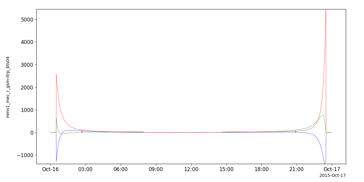
tts04('mms1_mec_r_gsm-itrp', parmod=params)

from pyspedas import tplot
tplot('mms1_mec_r_gsm-itrp_bts04')

Solar Wind Parameters

Note: This routine is provided as a convenience for users wishing to port IDL SPEDAS field line tracing code to PySPEDAS. In most cases, passing ‘autoload=True’ to the modeling or field line tracing routines, or using one of the model-specific routines described above in the “Managing model parameters” section, will be the easiest and cleanest way to prepare the model parameters.

To generate the “parmod” variable using Dst and solar wind data, use the get_tsy_params routine.

pyspedas.get_tsy_params(dst_tvar, imf_tvar, Np_tvar, Vp_tvar, model, pressure_tvar=None, newname=None, speed=False, g_variables=None)[source]

This procedure will interpolate inputs, generate Tsyganenko model parameters and store them in a tplot variable that can be passed directly to the model procedure.

Input

dst_tvar: str
tplot variable containing the Dst index

imf_tvar: str
tplot variable containing the interplanetary magnetic field vector in GSM coordinates

Np_tvar: str
tplot variable containing the solar wind ion density (cm**-3)

Vp_tvar: str
tplot variable containing the proton velocity

model: str
Tsyganenko model; should be: ‘T89’, T96’, ‘T01’,’TS04’

Parameters:

newname (str) – name of the output variable; default: t96_par, ‘t01_par’ or ‘ts04_par’, depending on the model
speed (bool) – Flag to indicate Vp_tvar is speed, and not velocity (defaults to False)
pressure_tvar (str) – Set this to specify a tplot variable containing solar wind dynamic pressure data. If not supplied, it will be calculated internally from proton density and proton speed.

returns:

Name of the tplot variable containing the parameters.

rtype:

str

Notes

The parameters are:

(1) solar wind pressure pdyn (nanopascals),
(2) dst (nanotesla),
(3) byimf,
(4) bzimf (nanotesla)
(5-10) indices w1 - w6, calculated as time integrals from the beginning of a storm

get_tsy_params Example

# load Dst and solar wind data
import pyspedas
pyspedas.projects.kyoto.dst(trange=['2015-10-16', '2015-10-17'])
pyspedas.projects.omni.data(trange=['2015-10-16', '2015-10-17'])

# join the components of B into a single variable
# BX isn't used
from pyspedas import join_vec
join_vec(['BX_GSE', 'BY_GSM', 'BZ_GSM'])

from pyspedas.get_tsy_params import get_tsy_params
params = get_tsy_params('kyoto_dst',
                     'BX_GSE-BY_GSM-BZ_GSM_joined',
                     'proton_density',
                     'flow_speed',
                     't96', # or 't01', 'ts04'
                     pressure_tvar='Pressure',
                     speed=True)

Field line tracing

PySPEDAS can perform field line tracing for any of the available models. As with the field models, the input to the field line tracing routines is a tplot variable containing the times and starting positions of each trace. The options for trace endpoints include tracing to the north ionosphere, the south ionosphere, or the field line “apex” or “equator” (the point where the radial component switches sign toward or away from Earth).

The field line traces are implemented as solutions to a differential equation initial value problem, using the solve_ivp method from the scipy library, with a Runge-Kutte order 4/5 solver. There is a single tracing routine ttrace2endpoint, where an ‘endpoint’ parameter (‘ionoshere-north’, ‘ionosphere-south’, or ‘equator’) determines which of the three endpoints to trace to. endpoint=’ionosphere-north’ or ‘ionosphere-south’ correspond to the IDL SPEDAS routine ttrace2iono, and endpoint=’equator’ corresponds to IDL SPEDAS ‘ttrace2equator’ routine.

The foot points and trace points returned by ttrace2endpoint will be in the GSM coordinate system by default. The foot_out_coord and trace_out_coord parameters can be used to specify different coordinate systems. For example, specifying foot_out_coord=’GEO’ will transform the foot points to GEO coordinates, which are easily converted to longitudes and latitudes suitable for plotting on maps. The default units will be Re (earth radii), but this can be changed via the foot_out_units and trace_out_units keyword parameters.

Previous versions of ttrace2endpoint used a boolean keyword argument ‘km’, to flag whether inputs and outputs should be in units of Re or km. The ‘km’ keyword is now deprecated; the equivalent functionality can be achieved, with greater flexibility, by using the units_in, foot_out_units, and trace_out_units keyword parameters.

pyspedas.ttrace2endpoint(tvar: str = None, model_str: str = None, endpoint: str = None, *, units_in: str = None, coord_in: str = None, foot_name: str = None, foot_out_coord: str = None, foot_out_units: str = 'Re', trace_name: str = None, trace_out_coord: str = None, trace_out_units: str = 'Re', bvec_name: str = None, diag_nevals_name: str = None, diag_reached_name: str = None, diag_s_max_name: str = None, diag_npts_name: str = None, parmod=None, kp=None, iopt=None, igrf_only=None, pdyn=None, dst=None, byimf=None, bzimf=None, g1=None, g2=None, w1=None, w2=None, w3=None, w4=None, w5=None, w6=None, autoload=False, km=None, r_iono_re: float = 1.0152561526870918, max_s: float = 200.0, max_step: float = 0.5, rtol: float = 1e-06, atol: float = 1e-09)[source]

Trace magnetic field lines to the north ionosphere, south ionosphere, or equator

Parameters:

tvar (str) – A tplot variable name specifying the times and start positions to be traced. Coordinates should be in GSM.
model_str (str) – A string specifying the field model to use. Valid options are ‘igrf’, ‘t89’, ‘t96’, ‘t01’, ‘t204’.
endpoint (str) – A string specifying the endpoint to trace to: ‘ionosphere-north’, ‘ionosphere-south’, or ‘equator’.
coord_in (str) – (Optional) Coordinate system of input variable, overrides any metadata in pos_var. Must be convertible to GSM.
units_in (str) – (Optional) Units of input variable, overrides any metadata in pos_var. Valid options: [‘km’, ‘Re’]
foot_name (str) – A string specifying the tplot variable to receive the foot point locations.
foot_out_coord (str) – (Optional) The desired coordinate system for the output foot points. If unspecified, output will be in GSM coordainates.
foot_out_units (str) – (Optional) Units of foot point variable to be returned. Valid options: [‘km’, ‘Re’] Default: ‘Re’
trace_name (str) – A string specifying the tplot variable to receive the trace points.
trace_out_coord (str) – (Optionsl) The desired coordinate system for the output trace points. If unspecified, output will be in GSM coordinates.
foot_out_units (str) – (Optional) Units of trace point variable to be returned. Valid options: [‘km’, ‘Re’] Default: ‘Re’
bvec_name (str) – A string specifying the tplot variable to receive the modeled field vectors at each trace point
diag_nevals_name (str) – A string specifying the tplot variable to receive the number of evaluations for each line traced.
diag_reached_name (str) – A string specifing the tplot variable to receive the status of each trace (1=endpoint reached, 0:gave up)
diag_s_max_name (str) – A string specifying the tplot variable to receive the path length (in Re) of each trace
diag_npts_name (str) – A string specifying the tplot variable to receive the number of points of each trace
parmod (Any) – A 10-element or nx10 element array (or equivalent tplot variable) of model parameter values
kp (Any) – The Kp parameter to use for the t89 model (scalar, array, or tplot variable name)
iopt (Any) – The model parameter to use for the t89 model (scalar, array, or tplot variable name)
igrf_only (bool) – For the t89 model, if true, only include the IGRF standard field.
pdyn (Any) – For the t96, t01, and ts04 models: solar wind dynamic pressure in nPa
dst (Any) – For the t96, t01, and ts04 models: Dst storm time index in nT
byimf (Any) – For the t96, t01, and ts04 models: Y component of interplanetary magnetic field
bzimf (Any) – for the t96, t01, and ts04 models: Z component of interplanetary magnetic field
g1 (Any) – For the t01 model: g1 index value
g2 (Any) – For the t01 model: g2 index value
w1 (Any) – For the ts04 models: w1 index value
w2 (Any) – For the ts04 models: w2 index value
w3 (Any) – For the ts04 models: w3 index value
w4 (Any) – For the ts04 models: w4 index value
w5 (Any) – For the ts04 models: w5 index value
w6 (Any) – For the ts04 models: w6 index value
km (bool) – (Optional) Override whatever units may be in the input variable metadata. If True, the input variable is assumed to be in units of km, otherwise Re. If false, the input units are determined from metadata. Deprecated: units_in, foot_out_units, and trace_out_units should be used instead.
autoload (boolean) – If true, automatically load model parameters from an appropriate data source.
max_s – Max path length in Re before giving up. Default: 200.0
max_step – Max RK45 step in Re. Default: 0.5
rtol, atol – Integrator tolerances (position units are Re). Defaults: 1e-6, 1e-9
r_iono_re – Ionosphere radius in Re. Default: 6468.4 / R_E_KM

Return type:

None

Examples

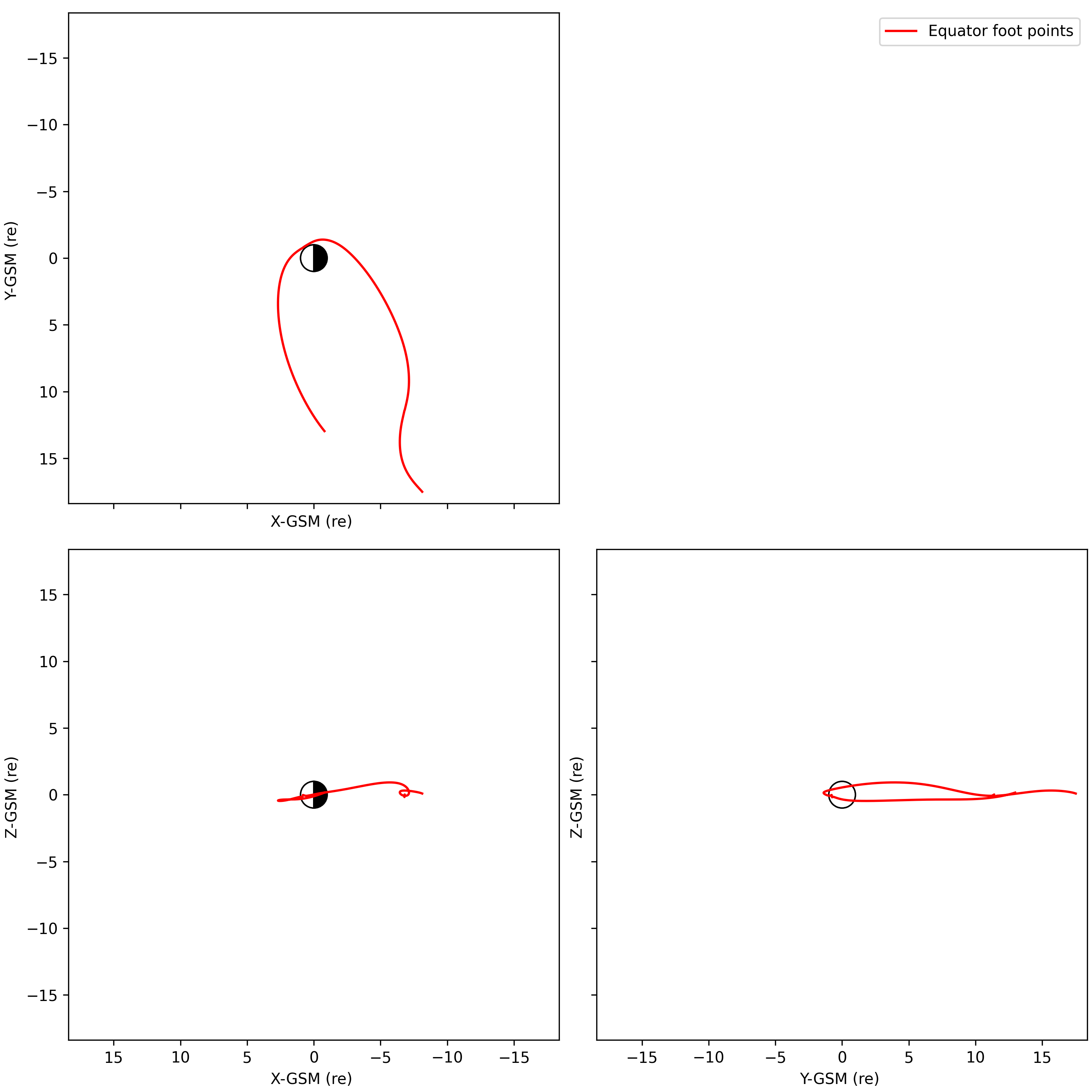
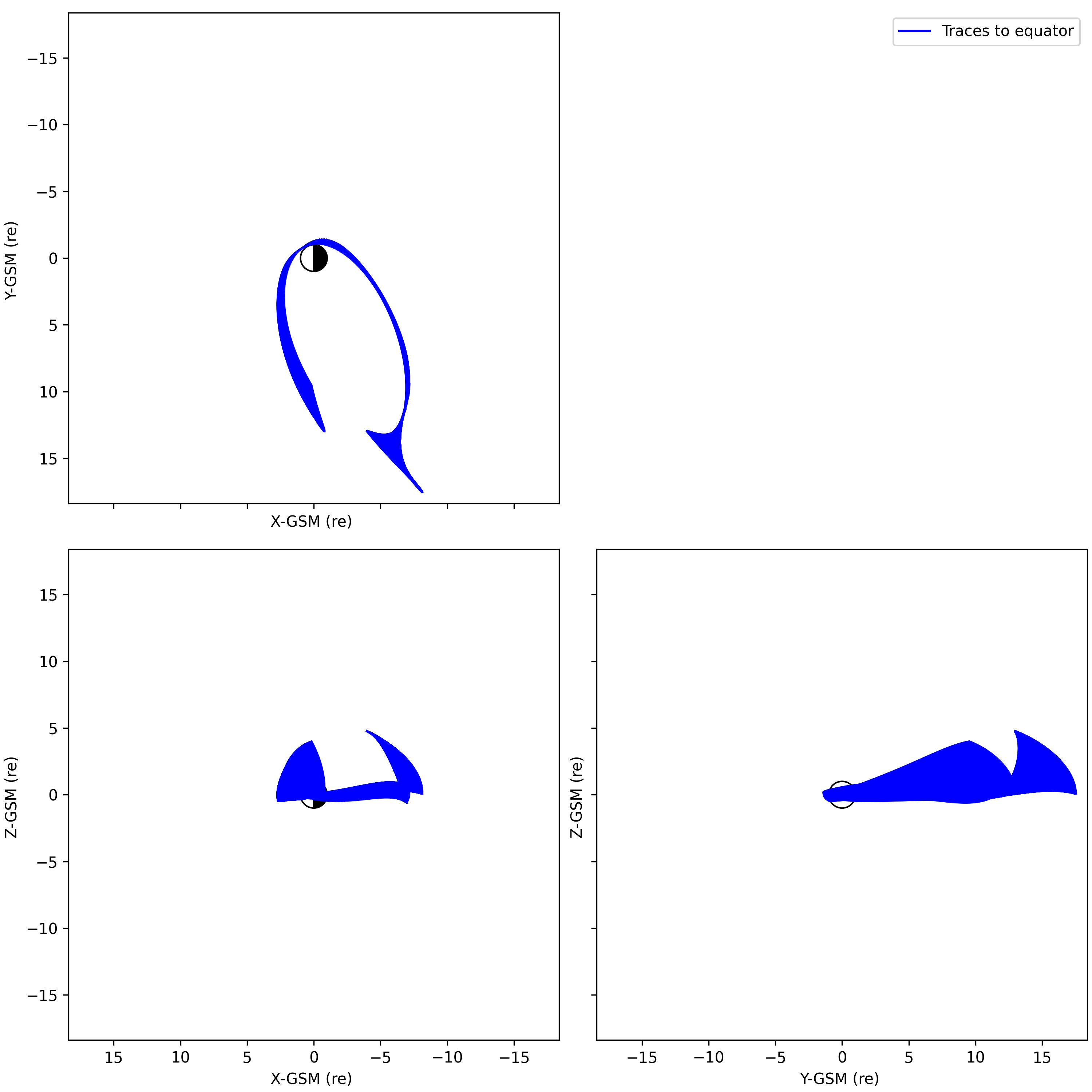
>>> from pyspedas.projects.themis import state
>>> from pyspedas import ttrace2endpoint, tplotxy3
>>> state(trange=['2007-03-23', '2007-03-23'], probe='a')
>>> # Trace to north ionosphere with T89 model, returning foot points and trace points in km
>>> ttrace2endpoint('tha_pos_gsm','t89','ionosphere-north',foot_name='ifoot89_n', trace_name='tha_trace_iono_n_t89', foot_out_units='km', trace_out_units='km')
>>> tplotxy3('ifoot89_n',legend_names=['North ionosphere foot points',], colors='red', reverse_x=True, show_centerbody=True,save_png='tha_iono_n_foot.png')
>>>
>>> # Trace to south ionosphere with T89 model. returning foot points and trace points in the default GSM coordinates, returning foot points and trace points in km
>>> ttrace2endpoint('tha_pos_gsm','t89','ionosphere-south',foot_name='ifoot89_s', trace_name='tha_trace_iono_s_t89', foot_out_units='km', trace_out_units='km')
>>> tplotxy3('ifoot89_s',legend_names=['South ionosphere foot points',], colors='red', reverse_x=True, show_centerbody=True,save_png='tha_iono_s_foot.png')
>>>
>>> # Trace to south ionosphere with T89 model. returning foot points in GEO coordinates and trace points in the default GSM coordinates, with units of km
>>> ttrace2endpoint('tha_pos_gsm','t89','ionosphere-south',foot_name='ifoot89_s', foot_out_coord='GEO', trace_name='tha_trace_iono_s_t89', foot_out_units='km', trace_out_units='km')
>>> tplotxy3('ifoot89_s',legend_names=['South ionosphere foot points',], colors='red', reverse_x=True, show_centerbody=True,save_png='tha_iono_s_foot_geo.png')
>>>
>>> # Trace to equator with T89 model, with foot points and trace points in units of km
>>> ttrace2endpoint('tha_pos_gsm','t89','equator',foot_name='eq_foot89', trace_name='tha_trace_equ_t89', foot_out_units='km', trace_out_units='km')
>>> tplotxy3('eq_foot89',legend_names=['Equator foot points'], colors='red', reverse_x=True, show_centerbody=True,save_png='tha_equ_foot.png')
>>> tplotxy3('tha_trace_equ_t89',legend_names=['Traces to equator'], colors='blue', reverse_x=True, show_centerbody=True, save_png='tha_equ_traces.png')

Field line tracing examples

from pyspedas.projects.themis import state
from pyspedas import ttrace2endpoint, tplotxy3
state(trange=['2007-03-23', '2007-03-23'], probe='a')
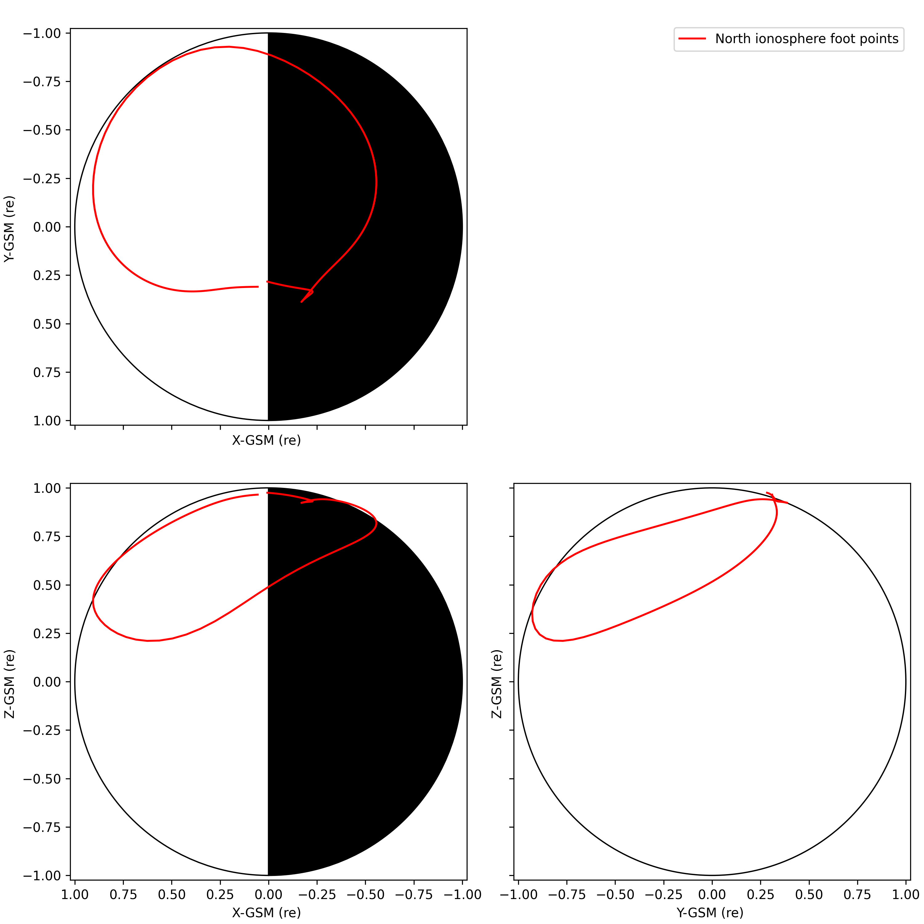
# Trace to north ionosphere with T89 model
ttrace2endpoint('tha_pos_gsm','t89','ionosphere-north',foot_name='ifoot89_n', trace_name='tha_trace_iono_n_t89', units_in='km', foot_out_units='km', trace_out_units='km')
tplotxy3('ifoot89_n',legend_names=['North ionosphere foot points',], colors='red', reverse_x=True, show_centerbody=True,save_png='tha_iono_n_foot.png')

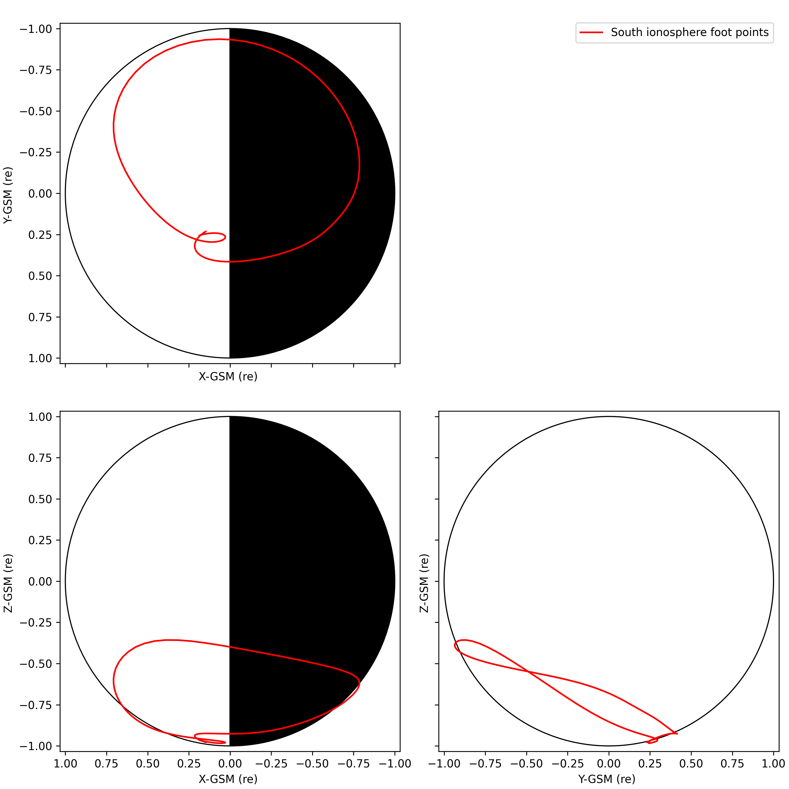
# Trace to south ionosphere with T89 model
ttrace2endpoint('tha_pos_gsm','t89','ionosphere-south',foot_name='ifoot89_s', trace_name='tha_trace_iono_s_t89', units_in='km', foot_out_units='km', trace_out_units='km')
tplotxy3('ifoot89_s',legend_names=['South ionosphere foot points',], colors='red', reverse_x=True, show_centerbody=True,save_png='tha_iono_s_foot.png')

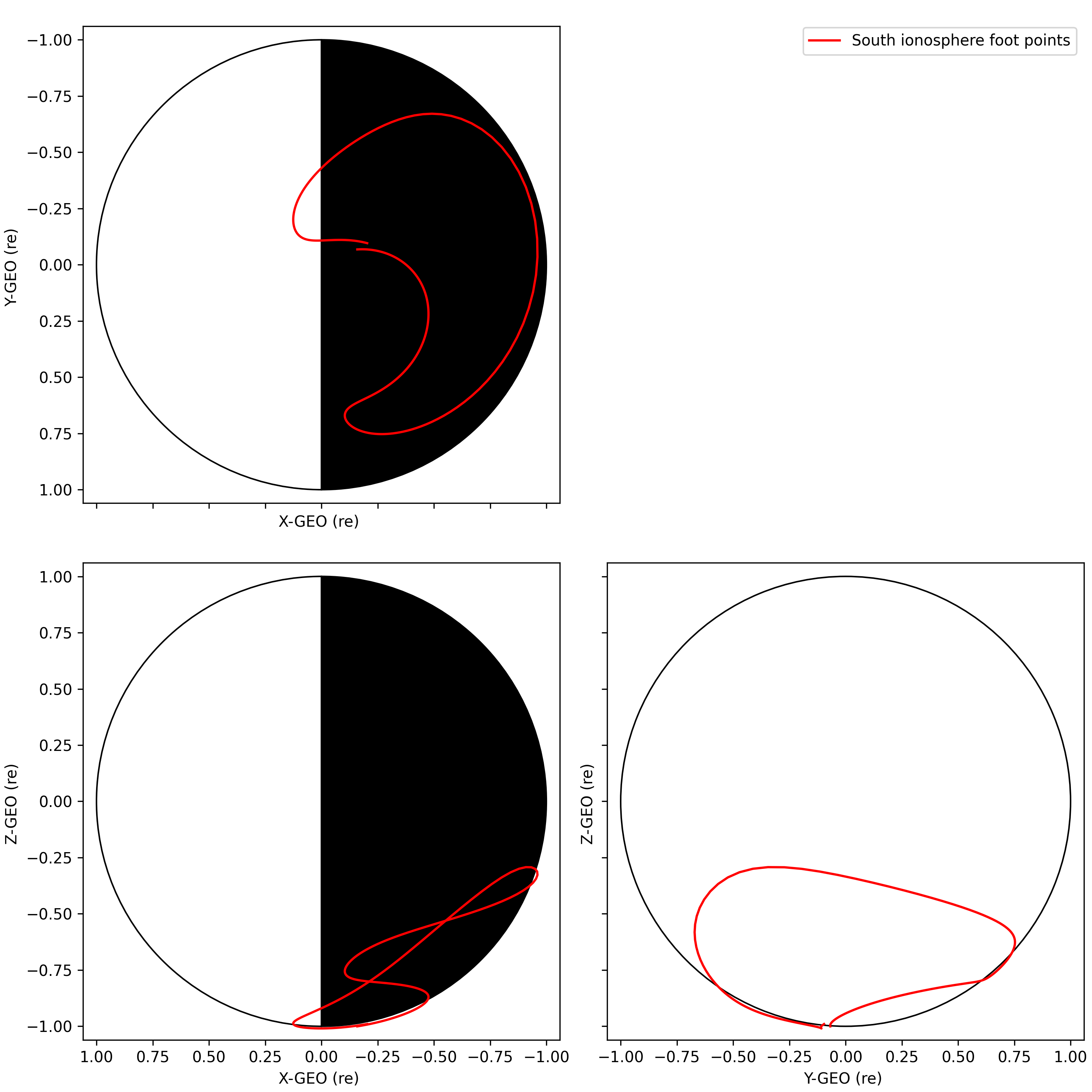
# Trace to south ionosphere with T89 model, returning the foot points in GEO coordinates
ttrace2endpoint('tha_pos_gsm','t89','ionosphere-south',foot_name='ifoot89_s', foot_out_coord='GEO', trace_name='tha_trace_iono_s_t89', units_in='km', foot_out_units='km', trace_out_units='km')
tplotxy3('ifoot89_s',legend_names=['South ionosphere foot points',], colors='red', reverse_x=True, show_centerbody=True,save_png='tha_iono_s_foot_geo.png')

# Trace to equator with T89 model
ttrace2endpoint('tha_pos_gsm','t89','equator',foot_name='eq_foot89', trace_name='tha_trace_equ_t89', units_in='km', foot_out_units='km', trace_out_units='km')
tplotxy3('eq_foot89',legend_names=['Equator foot points'], colors='red', reverse_x=True, show_centerbody=True,save_png='tha_equ_foot.png')
tplotxy3('tha_trace_equ_t89',legend_names=['Traces to equator'], colors='blue', reverse_x=True, show_centerbody=True, save_png='tha_equ_traces.png')

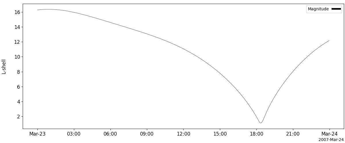
Calculating L-shell values

The L-shell of a given time and position is defined as the distance from Earth of the apex or equator of the field line passing through that point, in units of Earth radii (Re). This can be calculated with the PySPEDAS calculate_lshell routine.

pyspedas.calculate_lshell(pos_tvar: str, newname: str, units_in: str = None, coord_in: str = None)[source]

Calculate the L-shell values of a position variable

The L-shell represents the radial distance, in units of Re, of the apex of the field line passing through the input position.

Parameters:

pos_tvar (str)
Name of a tplot variable containing position data in GSM coordinates. It will be converted to units of Re if necessary.
units_in (str)
(Optional) Units of input variable. Overrides any units metadata that might be present. Valid values ([``’km’, ``'Re'] Default: None)
coord_in (str)
(Optional) Coordinate system of input variable. Overrides any coordinate system metadata that might be present. Valid values ([``’km’, ``'Re'] Default: None)
newname (str)
Name of new tplot variable containing L-shell values, derived by tracing to the equator
using the IGRF model.

Returns:

str
Name of the variable created.

Example

>>> from pyspedas.projects.themis import state
>>> from pyspedas import calculate_lshell, tplot
>>> state(trange=['2007-03-23', '2007-03-23'], probe='a')
>>> calculate_lshell('tha_pos_gsm','tha_pos_lshell')
>>> tplot('tha_pos_lshell')

L-shell example

from pyspedas.projects.themis import state
from pyspedas import calculate_lshell, tplot
state(trange=['2007-03-23', '2007-03-23'], probe='a')
calculate_lshell('tha_pos_gsm','tha_pos_lshell')
tplot('tha_pos_lshell')