Time History of Events and Macroscale Interactions during Substorms (THEMIS)

The routines in this module can be used to load data from the Time History of Events and Macroscale Interactions during Substorms (THEMIS) mission.

Fluxgate magnetometer (FGM)

pyspedas.projects.themis.fgm(trange=['2007-03-23', '2007-03-24'], probe='c', level='l2', suffix='', get_support_data=False, varformat=None, coord=None, varnames=[], downloadonly=False, notplot=False, no_update=False, time_clip=False)[source]

This function loads Fluxgate magnetometer (FGM) data

Parameters:

trange (list of str) – time range of interest [starttime, endtime] with the format ‘YYYY-MM-DD’,’YYYY-MM-DD’] or to specify more or less than a day [‘YYYY-MM-DD/hh:mm:ss’,’YYYY-MM-DD/hh:mm:ss’] Default: [‘2007-03-23’, ‘2007-03-24’]
probe (str or list of str) – Spacecraft probe letter(s) (‘a’, ‘b’, ‘c’, ‘d’ and/or ‘e’) Default: ‘c’
level (str) – Data level; Valid options: ‘l1’, ‘l2’ Default: ‘l2’
suffix (str) – The tplot variable names will be given this suffix. Default: no suffix
get_support_data (bool) – Data with an attribute “VAR_TYPE” with a value of “support_data” will be loaded into tplot. Default: False; only loads data with a “VAR_TYPE” attribute of “data”
varformat (str) – The file variable formats to load into tplot. Wildcard character “*” is accepted. Default: None; all variables are loaded
varnames (list of str) – List of variable names to load Default: Empty list, so all data variables are loaded
downloadonly (bool) – Set this flag to download the CDF files, but not load them into tplot variables Default: False
notplot (bool) – Return the data in hash tables instead of creating tplot variables Default: False
no_update (bool) – If set, only load data from your local cache Default: False
time_clip (bool) – Time clip the variables to exactly the range specified in the trange keyword Default: False

Returns:

List of tplot variables created Empty list if no data

Return type:

List of str

Example

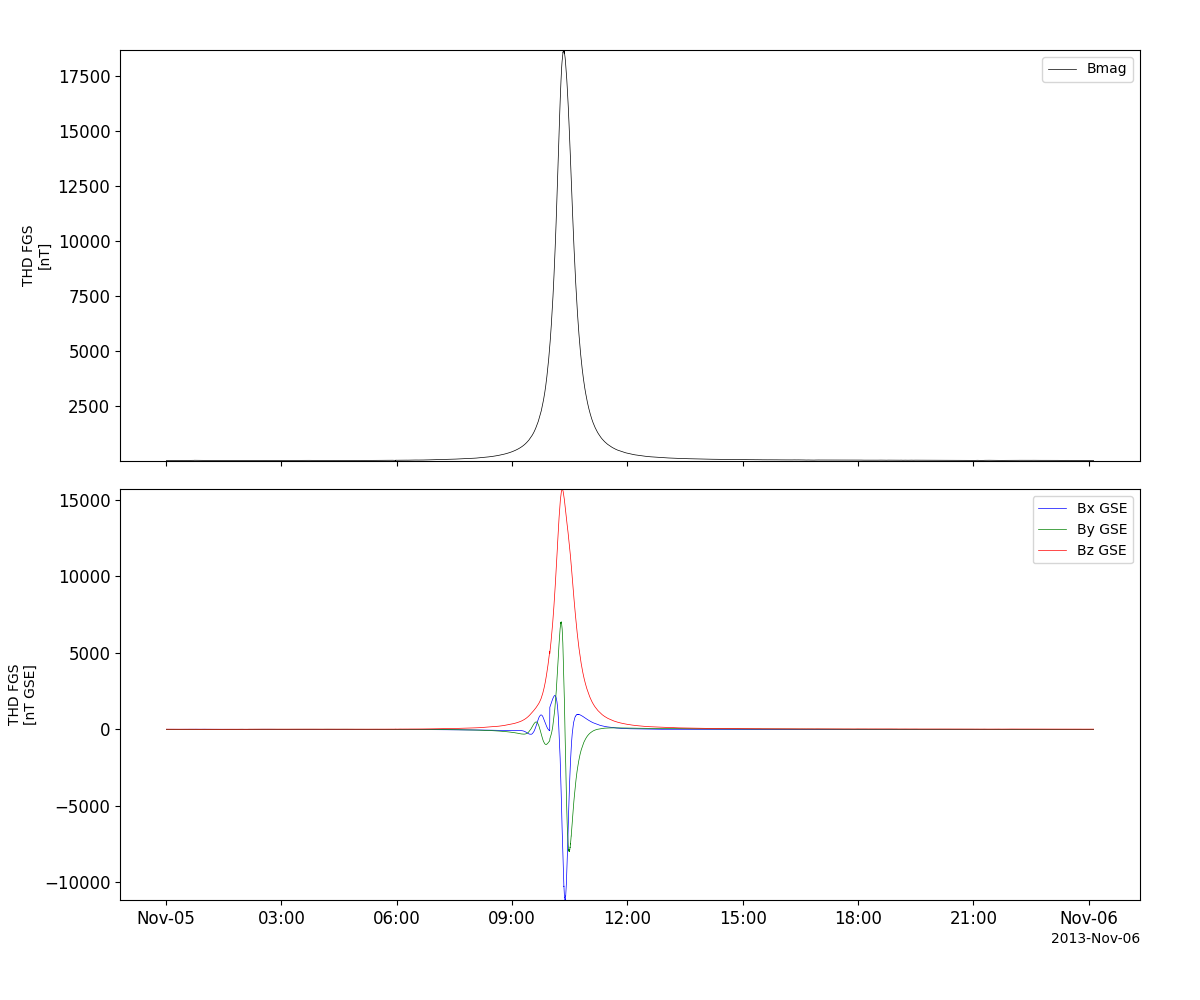
>>> import pyspedas
>>> from pyspedas import tplot
>>> fgm_vars = pyspedas.projects.themis.fgm(probe='d', trange=['2013-11-5', '2013-11-6'])
>>> tplot(['thd_fgs_btotal', 'thd_fgs_gse'])

Example

import pyspedas
from pyspedas import tplot
fgm_vars = pyspedas.projects.themis.fgm(probe='d', trange=['2013-11-5', '2013-11-6'])
tplot(['thd_fgs_btotal', 'thd_fgs_gse'])

Search-coil magnetometer (SCM)

pyspedas.projects.themis.scm(trange=['2007-03-23', '2007-03-24'], probe='c', level='l2', suffix='', get_support_data=False, varformat=None, varnames=[], downloadonly=False, notplot=False, no_update=False, time_clip=False)[source]

This function loads Search-coil magnetometer (SCM) data

Parameters:

trange (list of str) – time range of interest [starttime, endtime] with the format ‘YYYY-MM-DD’,’YYYY-MM-DD’] or to specify more or less than a day [‘YYYY-MM-DD/hh:mm:ss’,’YYYY-MM-DD/hh:mm:ss’] Default: [‘2007-03-23’, ‘2007-03-24’]
probe (str or list of str) – Spacecraft probe letter(s) (‘a’, ‘b’, ‘c’, ‘d’ and/or ‘e’) Default: ‘c’
level (str) – Data level; Valid options: ‘l1’, ‘l2’ Default: ‘l2’
suffix (str) – The tplot variable names will be given this suffix. Default: no suffix
get_support_data (bool) – Data with an attribute “VAR_TYPE” with a value of “support_data” will be loaded into tplot. Default: False; only loads data with a “VAR_TYPE” attribute of “data”
varformat (str) – The file variable formats to load into tplot. Wildcard character “*” is accepted. Default: None; all variables are loaded
varnames (list of str) – List of variable names to load Default: Empty list, so all data variables are loaded
downloadonly (bool) – Set this flag to download the CDF files, but not load them into tplot variables Default: False
notplot (bool) – Return the data in hash tables instead of creating tplot variables Default: False
no_update (bool) – If set, only load data from your local cache Default: False
time_clip (bool) – Time clip the variables to exactly the range specified in the trange keyword Default: False

Returns:

List of tplot variables created Empty list if no data

Return type:

List of str

Example

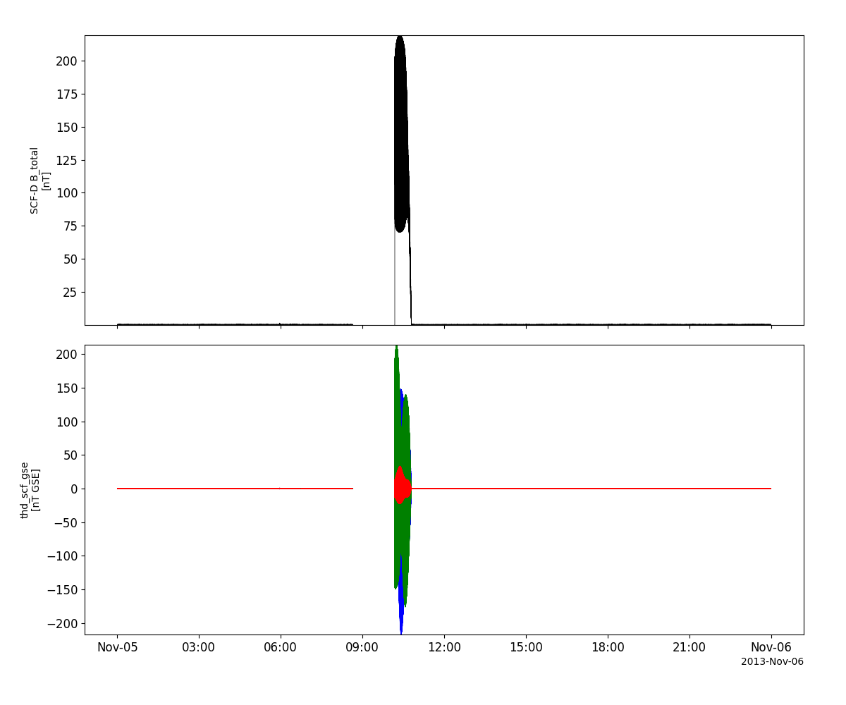
>>> import pyspedas
>>> from pyspedas import tplot
>>> scm_vars = pyspedas.projects.themis.scm(probe='d', trange=['2013-11-05', '2013-11-06'])
>>> tplot(['thd_scf_btotal', 'thd_scf_gse'])

Example

import pyspedas
from pyspedas import tplot
scm_vars = pyspedas.projects.themis.scm(probe='d', trange=['2013-11-5', '2013-11-6'])
tplot(['thd_scf_btotal', 'thd_scf_gse'])

Electric Field Instrument (EFI)

pyspedas.projects.themis.efi(trange=['2007-03-23', '2007-03-24'], probe='c', level='l2', datatype=None, suffix='', get_support_data=False, varformat=None, varnames=[], downloadonly=False, notplot=False, no_update=False, time_clip=False)[source]

This function loads Electric Field Instrument (EFI) data

Parameters:

trange (list of str) – time range of interest [starttime, endtime] with the format ‘YYYY-MM-DD’,’YYYY-MM-DD’] or to specify more or less than a day [‘YYYY-MM-DD/hh:mm:ss’,’YYYY-MM-DD/hh:mm:ss’] Default: [‘2007-03-23’, ‘2007-03-24’]
probe (str or list of str) – Spacecraft probe letter(s) (‘a’, ‘b’, ‘c’, ‘d’ and/or ‘e’) Default: ‘c’
level (str) – Processing level; Valid options: ‘l1’, ‘l2’ Default: ‘l2’

datatype (str or list of str) –

Data type; Valid L1 options:

'eff', Fast survey E12, E34, E56 waveforms
'efp', Particle burst E12, E34, E56 waveforms
'efw', Wave burst E12 E34, E56 waveforms
'vaf', Fast survey voltage group A, V1-V6 boom voltages
'vap', Particle burst voltage group A, V1-V6 boom voltages
'vaw', Wave burst voltage group A, V1-V6 boom voltages
'vbf', Fast survey voltage group B, V1-V6 boom voltages
'vbp', Particle burst voltage group B, V1-V6 boom voltages
'vbw', Wave burst voltage group B, V1-V6 boom voltages
L1 default: [eff. efp, efw, vaf. vap, vaw]

Valid L2 options:

'efi', Fast survey E field vectors and other quantities
'efp', Particle burst E field vectors
'efw', Wave burst E field vectors
L2 default: efi

suffix (str) – The tplot variable names will be given this suffix. Default: no suffix
get_support_data (bool) – Data with an attribute “VAR_TYPE” with a value of “support_data” will be loaded into tplot. Default: False; only loads data with a “VAR_TYPE” attribute of “data”
varformat (str) – The file variable formats to load into tplot. Wildcard character “*” is accepted. Default: None; all variables are loaded
varnames (list of str) – List of variable names to load Default: Empty list, so all data variables are loaded
downloadonly (bool) – Set this flag to download the CDF files, but not load them into tplot variables Default: False
notplot (bool) – Return the data in hash tables instead of creating tplot variables Default: False
no_update (bool) – If set, only load data from your local cache Default: False
time_clip (bool) – Time clip the variables to exactly the range specified in the trange keyword Default: False

Returns:

List of tplot variables created Empty list if no data

Return type:

List of str

Example

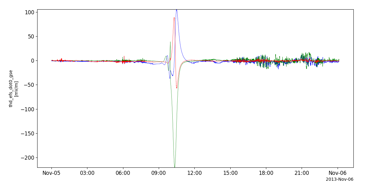
>>> import pyspedas
>>> from pyspedas import tplot
>>> efi_vars = pyspedas.projects.themis.efi(probe='d', trange=['2013-11-5', '2013-11-6'])
>>> tplot('thd_efs_dot0_gse')

Example

import pyspedas
from pyspedas import tplot
efi_vars = pyspedas.projects.themis.efi(probe='d', trange=['2013-11-5', '2013-11-6'])
tplot('thd_efs_dot0_gse')

Electrostatic Analyzer (ESA)

pyspedas.projects.themis.esa(trange=['2007-03-23', '2007-03-24'], probe='c', level='l2', suffix='', get_support_data=False, varformat=None, varnames=[], downloadonly=False, notplot=False, no_update=False, time_clip=False)[source]

This function loads Electrostatic Analyzer (ESA) data

Parameters:

trange (list of str) – time range of interest [starttime, endtime] with the format ‘YYYY-MM-DD’,’YYYY-MM-DD’] or to specify more or less than a day [‘YYYY-MM-DD/hh:mm:ss’,’YYYY-MM-DD/hh:mm:ss’] Default: [‘2007-03-23’, ‘2007-03-24’]
probe (str or list of str) – Spacecraft probe letter(s) (‘a’, ‘b’, ‘c’, ‘d’ and/or ‘e’) Default: ‘c’
level (str) – Data level; Valid options: ‘l1’, ‘l2’ Default: ‘l2’
suffix (str) – The tplot variable names will be given this suffix. Default: no suffix
get_support_data (bool) – Data with an attribute “VAR_TYPE” with a value of “support_data” will be loaded into tplot. Default: False; only loads data with a “VAR_TYPE” attribute of “data”
varformat (str) – The file variable formats to load into tplot. Wildcard character “*” is accepted. Default: None; all variables are loaded
varnames (list of str) – List of variable names to load Default: Empty list, so all data variables are loaded
downloadonly (bool) – Set this flag to download the CDF files, but not load them into tplot variables Default: False
notplot (bool) – Return the data in hash tables instead of creating tplot variables Default: False
no_update (bool) – If set, only load data from your local cache Default: False
time_clip (bool) – Time clip the variables to exactly the range specified in the trange keyword Default: False

Returns:

List of tplot variables created Empty list if no data

Return type:

List of str

Example

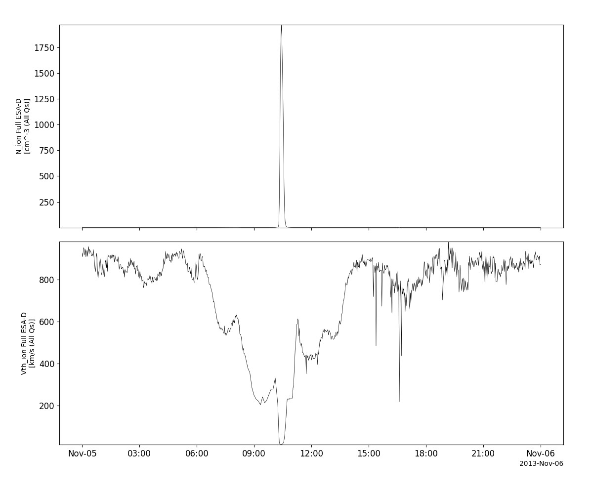
>>> import pyspedas
>>> from pyspedas import tplot
>>> esa_vars = pyspedas.projects.themis.esa(probe='d', trange=['2013-11-5', '2013-11-6'])
>>> tplot(['thd_peif_density', 'thd_peif_vthermal'])

Example

import pyspedas
from pyspedas import tplot
esa_vars = pyspedas.projects.themis.esa(probe='d', trange=['2013-11-5', '2013-11-6'])
tplot(['thd_peif_density', 'thd_peif_vthermal'])

Solid State Telescope (SST)

pyspedas.projects.themis.sst(trange=['2007-03-23', '2007-03-24'], probe='c', level='l2', suffix='', get_support_data=False, varformat=None, varnames=[], downloadonly=False, notplot=False, no_update=False, time_clip=False)[source]

This function loads Solid State Telescope (SST) data

Parameters:

trange (list of str) – time range of interest [starttime, endtime] with the format ‘YYYY-MM-DD’,’YYYY-MM-DD’] or to specify more or less than a day [‘YYYY-MM-DD/hh:mm:ss’,’YYYY-MM-DD/hh:mm:ss’] Default: [‘2007-03-23’, ‘2007-03-24’]
probe (str or list of str) – Spacecraft probe letter(s) (‘a’, ‘b’, ‘c’, ‘d’ and/or ‘e’) Default: ‘c’
level (str) – Data level; Valid options: ‘l1’, ‘l2’ Default: ‘l2’
suffix (str) – The tplot variable names will be given this suffix. Default: no suffix
get_support_data (bool) – Data with an attribute “VAR_TYPE” with a value of “support_data” will be loaded into tplot. Default: False; only loads data with a “VAR_TYPE” attribute of “data”
varformat (str) – The file variable formats to load into tplot. Wildcard character “*” is accepted. Default: None; all variables are loaded
varnames (list of str) – List of variable names to load Default: Empty list, so all data variables are loaded
downloadonly (bool) – Set this flag to download the CDF files, but not load them into tplot variables Default: False
notplot (bool) – Return the data in hash tables instead of creating tplot variables Default: False
no_update (bool) – If set, only load data from your local cache Default: False
time_clip (bool) – Time clip the variables to exactly the range specified in the trange keyword Default: False

Returns:

List of tplot variables created Empty list if no data

Return type:

List of str

Notes

The thx_*_atten variables produced when loading SST L1 data contain 4 status bits, representing the state of the attenuators on the two SST sensor heads, defined as:

(MSB) Open Equatorial Attenuator,
Closed Equatorial Attenuator,
Open Polar Attenuator,
(LSB) Closed Polar Attenuator

With MSB/LSB not representing actual bits, but as labels to clarify bit order. Some examples:

0x5: both attenuators closed
0xA: both attenuators open
0x6: equatorial closed, polar open  (Occurs during stuck atten error on themis D)
0xf: Error state. Invalid data.
0x9: equatorial open, polar closed (This should never actually happen)

Example

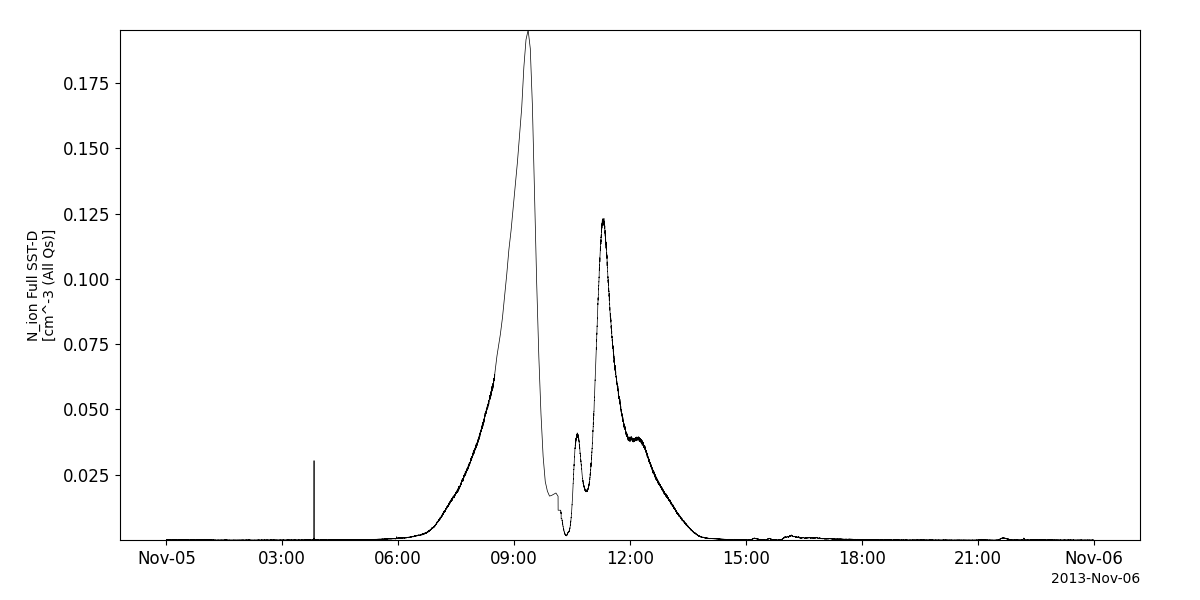
>>> import pyspedas
>>> from pyspedas import tplot
>>> sst_vars = pyspedas.projects.themis.sst(probe='d', trange=['2013-11-5', '2013-11-6'])
>>> tplot('thd_psif_density')

Example

import pyspedas
from pyspedas import tplot
sst_vars = pyspedas.projects.themis.sst(probe='d', trange=['2013-11-5', '2013-11-6'])
tplot('thd_psif_density')

Onboard Filter Bank Data (FBK)

pyspedas.projects.themis.fbk(trange=['2007-03-23', '2007-03-24'], probe='c', level='l2', suffix='', get_support_data=False, varformat=None, varnames=[], downloadonly=False, notplot=False, no_update=False, time_clip=False)[source]

This function loads THEMIS FBK data

Parameters:

trange – list of str time range of interest [starttime, endtime] with the format ‘YYYY-MM-DD’,’YYYY-MM-DD’] or to specify more or less than a day [‘YYYY-MM-DD/hh:mm:ss’,’YYYY-MM-DD/hh:mm:ss’] Default: [‘2007-03-23’, ‘2007-03-24’]
probe – str or list of str Spacecraft probe letter(s) (‘a’, ‘b’, ‘c’, ‘d’ and/or ‘e’) Default: ‘c’
level – str Data level; Valid options: ‘l1’, ‘l2’ Default: ‘l2’
level – str Data level; Valid options: ‘l1’, ‘l2’ Default: ‘l2’
suffix – str The tplot variable names will be given this suffix. Default: no suffix
get_support_data – bool Data with an attribute “VAR_TYPE” with a value of “support_data” will be loaded into tplot. Default: False; only loads data with a “VAR_TYPE” attribute of “data”
varformat – str The file variable formats to load into tplot. Wildcard character “*” is accepted. Default: None; all variables are loaded
varnames – list of str List of variable names to load Default: Empty list, so all data variables are loaded
downloadonly – bool Set this flag to download the CDF files, but not load them into tplot variables Default: False
notplot – bool Return the data in hash tables instead of creating tplot variables Default: False
no_update – bool If set, only load data from your local cache Default: False
time_clip – bool Time clip the variables to exactly the range specified in the trange keyword Default: False

Returns:

List of tplot variables created Empty list if no data

Return type:

List of str

Example

>>> import pyspedas
>>> from pyspedas import tplot
>>> fbk_vars = pyspedas.projects.themis.fbk(probe='d', trange=['2013-11-5', '2013-11-6'])
>>> tplot(['thd_fb_edc12', 'thd_fb_scm1'])

Onboard FFT Data (FFT)

pyspedas.projects.themis.fft(trange=['2007-03-23', '2007-03-24'], probe='c', level='l2', suffix='', get_support_data=False, varformat=None, varnames=[], downloadonly=False, notplot=False, no_update=False, time_clip=False)[source]

This function loads THEMIS FFT data

Parameters:

trange (list of str) – time range of interest [starttime, endtime] with the format ‘YYYY-MM-DD’,’YYYY-MM-DD’] or to specify more or less than a day [‘YYYY-MM-DD/hh:mm:ss’,’YYYY-MM-DD/hh:mm:ss’] Default: [‘2007-03-23’, ‘2007-03-24’]
probe (str or list of str) – Spacecraft probe letter(s) (‘a’, ‘b’, ‘c’, ‘d’ and/or ‘e’) Default: ‘c’
level (str) – Data level; Valid options: ‘l1’, ‘l2’ Default: ‘l2’
suffix (str) – The tplot variable names will be given this suffix. Default: no suffix
get_support_data (bool) – Data with an attribute “VAR_TYPE” with a value of “support_data” will be loaded into tplot. Default: False; only loads data with a “VAR_TYPE” attribute of “data”
varformat (str) – The file variable formats to load into tplot. Wildcard character “*” is accepted. Default: None; all variables are loaded
varnames (list of str) – List of variable names to load Default: Empty list, so all data variables are loaded
downloadonly (bool) – Set this flag to download the CDF files, but not load them into tplot variables Default: False
notplot (bool) – Return the data in hash tables instead of creating tplot variables Default: False
no_update (bool) – If set, only load data from your local cache Default: False
time_clip (bool) – Time clip the variables to exactly the range specified in the trange keyword Default: False

Returns:

List of tplot variables created Empty list if no data

Return type:

List of str

Example

>>> import pyspedas
>>> from pyspedas import tplot
>>> fft_vars = pyspedas.projects.themis.fft(probe='d', trange=['2013-11-5', '2013-11-6'])
>>> tplot(['thd_fff_32_edc12','thd_fff_32_scm2'])

Onboard Moments Data (MOM)

pyspedas.projects.themis.mom(trange=['2008-03-23', '2008-03-24'], probe='c', level='l2', suffix='', get_support_data=False, varformat=None, varnames=[], downloadonly=False, notplot=False, no_update=False, time_clip=False)[source]

This function loads THEMIS moments data

Parameters:

trange (list of str) – time range of interest [starttime, endtime] with the format ‘YYYY-MM-DD’,’YYYY-MM-DD’] or to specify more or less than a day [‘YYYY-MM-DD/hh:mm:ss’,’YYYY-MM-DD/hh:mm:ss’] Default: [‘2008-03-23’, ‘2008-03-24’]
probe (str or list of str) – Spacecraft probe letter(s) (‘a’, ‘b’, ‘c’, ‘d’ and/or ‘e’) Default: ‘c’
level (str) – Data level; Valid options: ‘l1’, ‘l2’ Default: ‘l2’
level (str) – Data level; Valid options: ‘l2’ Default: ‘l2’
suffix (str) – The tplot variable names will be given this suffix. Default: no suffix
get_support_data (bool) – Data with an attribute “VAR_TYPE” with a value of “support_data” will be loaded into tplot. Default: False; only loads data with a “VAR_TYPE” attribute of “data”
varformat (str) – The file variable formats to load into tplot. Wildcard character “*” is accepted. Default: None; all variables are loaded
varnames (list of str) – List of variable names to load Default: Empty list, so all data variables are loaded
downloadonly (bool) – Set this flag to download the CDF files, but not load them into tplot variables Default: False
notplot (bool) – Return the data in hash tables instead of creating tplot variables Default: False
no_update (bool) – If set, only load data from your local cache Default: False
time_clip (bool) – Time clip the variables to exactly the range specified in the trange keyword Default: False

Returns:

List of tplot variables created Empty list if no data

Return type:

List of str

Example

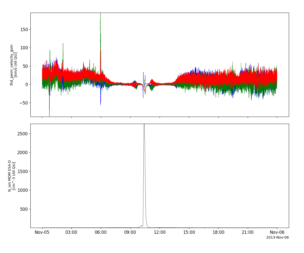
>>> import pyspedas
>>> from pyspedas import tplot
>>> mom_vars = pyspedas.projects.themis.mom(probe='d', trange=['2013-11-5', '2013-11-6'])
>>> tplot(['thd_peim_velocity_gsm', 'thd_peim_density'])

Example

import pyspedas
from pyspedas import tplot
mom_vars = pyspedas.projects.themis.mom(probe='d', trange=['2013-11-5', '2013-11-6'])
tplot(['thd_peim_velocity_gsm', 'thd_peim_density'])

Ground computed moments data (GMOM)

pyspedas.projects.themis.gmom(trange=['2007-03-23', '2007-03-24'], probe='c', level='l2', suffix='', get_support_data=False, varformat=None, varnames=[], downloadonly=False, notplot=False, no_update=False, time_clip=False)[source]

This function loads THEMIS Level 2 ground calculated combined ESA+SST moments.

Parameters:

trange (list of str) – time range of interest [starttime, endtime] with the format ‘YYYY-MM-DD’,’YYYY-MM-DD’] or to specify more or less than a day [‘YYYY-MM-DD/hh:mm:ss’,’YYYY-MM-DD/hh:mm:ss’] Default: [‘2007-03-23’, ‘2007-03-24’]
probe (str or list of str) – Spacecraft probe letter(s) (‘a’, ‘b’, ‘c’, ‘d’ and/or ‘e’) Default: ‘c’
level (str) – Data level; Valid options: ‘l2’ Default: ‘l2’
suffix (str) – The tplot variable names will be given this suffix. Default: no suffix
get_support_data (bool) – Data with an attribute “VAR_TYPE” with a value of “support_data” will be loaded into tplot. Default: False; only loads data with a “VAR_TYPE” attribute of “data”
varformat (str) – The file variable formats to load into tplot. Wildcard character “*” is accepted. Default: None; all variables are loaded
varnames (list of str) – List of variable names to load Default: Empty list, so all data variables are loaded
downloadonly (bool) – Set this flag to download the CDF files, but not load them into tplot variables Default: False
notplot (bool) – Return the data in hash tables instead of creating tplot variables Default: False
no_update (bool) – If set, only load data from your local cache Default: False
time_clip (bool) – Time clip the variables to exactly the range specified in the trange keyword Default: False

Returns:

List of tplot variables created Empty list if no data

Return type:

List of str

Example

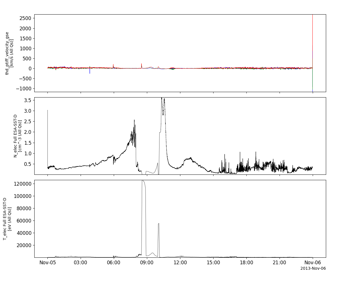
>>> import pyspedas
>>> from pyspedas import tplot
>>> gmom_vars = pyspedas.projects.themis.gmom(probe='d', trange=['2013-11-5', '2013-11-6'])
>>> tplot(['thd_ptiff_velocity_gse', 'thd_pteff_density', 'thd_pteff_avgtemp'])

Example

import pyspedas
from pyspedas import tplot
gmom_vars = pyspedas.projects.themis.gmom(probe='d', trange=['2013-11-5', '2013-11-6'])
tplot(['thd_ptiff_velocity_gse', 'thd_pteff_density', 'thd_pteff_avgtemp'])

State data (STATE)

pyspedas.projects.themis.state(trange=['2007-03-23', '2007-03-24'], probe='c', level='l1', suffix='', get_support_data=False, varformat=None, exclude_format=None, varnames=[], downloadonly=False, notplot=False, no_update=False, time_clip=False, keep_spin=False)[source]

Load THEMIS state data

Parameters:

trange (list of str) – time range of interest [starttime, endtime] with the format [‘YYYY-MM-DD’,’YYYY-MM-DD’] or to specify more or less than a day [‘YYYY-MM-DD/hh:mm:ss’,’YYYY-MM-DD/hh:mm:ss’] Default: [‘2007-03-23’, ‘2007-03-24’]
probe (str or list of str) – Spacecraft probe letter(s) (‘a’, ‘b’, ‘c’, ‘d’ and/or ‘e’) Default: ‘c’
level (str) – Data type; Valid options: ‘l1’ Default: ‘l1’
suffix (str) – The tplot variable names will be given this suffix. Default: None
get_support_data (bool) – Data with an attribute “VAR_TYPE” with a value of “support_data” will be loaded into tplot. Default: False
varformat (str) – The file variable formats to load into tplot. Wildcard character “*” is accepted. By default, all variables are loaded in. Default: None (all variables are loaded)
exclude_format (str) – If specified, CDF variables matching this pattern will not be processed. Wildcard character “*” is accepted. Default: None
varnames (list of str) – List of variable names to load. If list is empty or unsoecified, all data variables are loaded Default: [] (all variables are loaded)
downloadonly (bool) – Set this flag to download the CDF files, but not load them into tplot variables Default: false
notplot (bool) – Return the data in hash tables instead of creating tplot variables Default: false
no_update (bool) – If set, only load data from your local cache Default: false
time_clip (bool) – Time clip the variables to exactly the range specified in the trange keyword Default: false
keep_spin (bool) – If True, do not delete the spin model tplot variables after the spin models are built. Default: False

Returns:

List of str
List of tplot variables created
Empty list if no data loaded

Example

>>> import pyspedas
>>> from pyspedas import tplot
>>> pyspedas.projects.themis.state(trange=['2007-03-23', '2007-03-24'], probe='a', varnames=['tha_pos_gse','tha_vel_gse'])
>>> tplot['tha_pos_gse', 'tha_vel_gse'])

Example

import pyspedas
from pyspedas import tplot
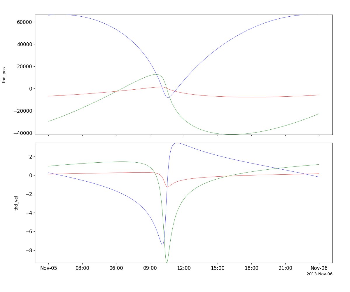
state_vars = pyspedas.projects.themis.state(probe='d', trange=['2013-11-5', '2013-11-6'])
tplot(['thd_pos', 'thd_vel'])

Orbit data from SSCWeb (SSC)

pyspedas.projects.themis.ssc(trange=['2017-03-23', '2017-03-24'], probe='c', level='l2', suffix='', get_support_data=False, varformat=None, varnames=[], downloadonly=False, notplot=False, no_update=False, time_clip=True)[source]

Load THEMIS current/past orbit data from CDAWeb/SSCWeb (Satellite Situation Center).

For example: https://cdaweb.gsfc.nasa.gov/pub/data/themis/thc/ssc/

See also, pyspedas.projects.themis.state_tools.ssc_pre

Parameters:

trange (list of str) – time range of interest [starttime, endtime] with the format ‘YYYY-MM-DD’,’YYYY-MM-DD’] or to specify more or less than a day [‘YYYY-MM-DD/hh:mm:ss’,’YYYY-MM-DD/hh:mm:ss’] Default: [‘2017-03-23’, ‘2017-03-24’]
probe (str or list of str) – Spacecraft probe letter(s) (‘a’, ‘b’, ‘c’, ‘d’ and/or ‘e’) Default: ‘c’
level (str) – Data type; Default: ‘l2’; Unused.
suffix (str) – The tplot variable names will be given this suffix. Default: no suffix
get_support_data (bool) – Data with an attribute “VAR_TYPE” with a value of “support_data” will be loaded into tplot. Default: False; only loads data with a “VAR_TYPE” attribute of “data”
varformat (str) – The file variable formats to load into tplot. Wildcard character “*” is accepted. Default: None; all variables are loaded
varnames (list of str) – List of variable names to load Default: Empty list, so all data variables are loaded
downloadonly (bool) – Set this flag to download the CDF files, but not load them into tplot variables Default: False
notplot (bool) – Return the data in hash tables instead of creating tplot variables Default: False
no_update (bool) – If set, only load data from your local cache Default: False
time_clip (bool) – Time clip the variables to exactly the range specified in the trange keyword Default: True

Returns:

List of tplot variables created Empty list if no data

Return type:

List of str

Example

>>> from pyspedas.projects.themis import ssc
>>> vars = ssc(probe='d', trange=['2013-11-5', '2013-11-6'])
>>> print(vars)

Example

from pyspedas.projects.themis import ssc
ssc_vars = ssc(probe='d', trange=['2012-10-01', '2012-10-02'])
print(ssc_vars)

['GEO_LAT', 'GEO_LON', 'GEO_LCT_T', 'GM_LAT', 'GM_LON', 'GM_LCT_T', 'GSE_LAT', 'GSE_LON', 'GSE_LCT_T', 'GSM_LAT', 'GSM_LON', 'SM_LAT', 'SM_LON', 'SM_LCT_T', 'NorthBtrace_GEO_LAT', 'NorthBtrace_GEO_LON', 'NorthBtrace_GEO_ARCLEN', 'SouthBtrace_GEO_LAT', 'SouthBtrace_GEO_LON', 'SouthBtrace_GEO_ARCLEN', 'NorthBtrace_GM_LAT', 'NorthBtrace_GM_LON', 'NorthBtrace_GM_ARCLEN', 'SouthBtrace_GM_LAT', 'SouthBtrace_GM_LON', 'SouthBtrace_GM_ARCLEN', 'RADIUS', 'MAG_STRTH', 'DNEUTS', 'BOW_SHOCK', 'MAG_PAUSE', 'L_VALUE', 'INVAR_LAT', 'MAG_X', 'MAG_Y', 'MAG_Z', 'XYZ_GEO', 'XYZ_GM', 'XYZ_GSE', 'XYZ_GSM', 'XYZ_SM']

Orbit predictions from SSCWeb (SSC_PRE)

pyspedas.projects.themis.ssc_pre(trange=['2026-03-23', '2026-03-24'], probe='c', level='l2', suffix='', get_support_data=False, varformat=None, varnames=[], downloadonly=False, notplot=False, no_update=False, time_clip=True)[source]

Load THEMIS predicted orbit data from CDAWeb/SSCWeb (Satellite Situation Center).

For example: https://cdaweb.gsfc.nasa.gov/pub/data/themis/thc/ssc_pre/ Each downloaded file contains data for a full year.

See also, pyspedas.projects.themis.state_tools.ssc

Parameters:

trange (list of str) – time range of interest [starttime, endtime] with the format ‘YYYY-MM-DD’,’YYYY-MM-DD’] or to specify more or less than a day [‘YYYY-MM-DD/hh:mm:ss’,’YYYY-MM-DD/hh:mm:ss’] Default: [‘2017-03-23’, ‘2017-03-24’]
probe (str or list of str) – Spacecraft probe letter(s) (‘a’, ‘b’, ‘c’, ‘d’ and/or ‘e’) Default: ‘c’
level (str) – Data type; Default: ‘l2’; Unused.
suffix (str) – The tplot variable names will be given this suffix. Default: no suffix
get_support_data (bool) – Data with an attribute “VAR_TYPE” with a value of “support_data” will be loaded into tplot. Default: False; only loads data with a “VAR_TYPE” attribute of “data”
varformat (str) – The file variable formats to load into tplot. Wildcard character “*” is accepted. Default: None; all variables are loaded
varnames (list of str) – List of variable names to load Default: Empty list, so all data variables are loaded
downloadonly (bool) – Set this flag to download the CDF files, but not load them into tplot variables Default: False
notplot (bool) – Return the data in hash tables instead of creating tplot variables Default: False
no_update (bool) – If set, only load data from your local cache Default: False
time_clip (bool) – Time clip the variables to exactly the range specified in the trange keyword Default: True

Returns:

List of tplot variables created Empty list if no data

Return type:

List of str

Example

>>> from pyspedas.projects.themis import ssc_pre
>>> vars = ssc_pre(probe='d', trange=['2026-12-25', '2026-12-26'])
>>> print(vars)

Example

from pyspedas.projects.themis import ssc_pre
ssc_pre_vars = ssc_pre(probe='a', trange=['2028-12-01', '2028-12-02'])
print(ssc_pre_vars)

['GEO_LAT', 'GEO_LON', 'GEO_LCT_T', 'GM_LAT', 'GM_LON', 'GM_LCT_T', 'GSE_LAT', 'GSE_LON', 'GSE_LCT_T', 'GSM_LAT', 'GSM_LON', 'SM_LAT', 'SM_LON', 'SM_LCT_T', 'NorthBtrace_GEO_LAT', 'NorthBtrace_GEO_LON', 'NorthBtrace_GEO_ARCLEN', 'SouthBtrace_GEO_LAT', 'SouthBtrace_GEO_LON', 'SouthBtrace_GEO_ARCLEN', 'NorthBtrace_GM_LAT', 'NorthBtrace_GM_LON', 'NorthBtrace_GM_ARCLEN', 'SouthBtrace_GM_LAT', 'SouthBtrace_GM_LON', 'SouthBtrace_GM_ARCLEN', 'RADIUS', 'MAG_STRTH', 'DNEUTS', 'BOW_SHOCK', 'MAG_PAUSE', 'L_VALUE', 'INVAR_LAT', 'MAG_X', 'MAG_Y', 'MAG_Z', 'XYZ_GEO', 'XYZ_GM', 'XYZ_GSE', 'XYZ_GSM', 'XYZ_SM']

Ground Magnetometer Data (GMAG)

pyspedas.projects.themis.gmag(trange=['2007-03-23', '2007-03-24'], sites=None, group=None, level='l2', prefix='', suffix='', get_support_data=False, varformat=None, varnames=[], downloadonly=False, notplot=False, no_update=False, time_clip=False, force_download=False, sampling_rate=1)[source]

Load ground magnetometer data from the THEMIS mission.

Parameters:

trange (list, optional) – Time range of interest in the format [“start_date”, “end_date”]. Default is [“2007-03-23”, “2007-03-24”].
sites (list or str, optional) – List of ground magnetometer sites to load data for. If None, data for all available sites will be loaded. Default is None.
group (str, optional) – Name of a pre-defined group of sites to load data for. If specified, the ‘sites’ parameter will be ignored. Default is None.
level (str, optional) – Data level to load. Default is “l2”.
prefix (str, optional) – Prefix to append to the variable names. Default is “”.
suffix (str, optional) – Suffix to append to the variable names. Default is “”.
get_support_data (bool, optional) – Flag indicating whether to download support data. Default is False.
varformat (str, optional) – Format of the variable names. Default is None.
varnames (list, optional) – List of specific variable names to load. Default is [].
downloadonly (bool, optional) – Flag indicating whether to only download the data without loading it. Default is False.
notplot (bool, optional) – Flag indicating whether to plot the loaded data. Default is False.
no_update (bool, optional) – Flag indicating whether to update the data files. Default is False.
time_clip (bool, optional) – Flag indicating whether to clip the data to the specified time range. Default is False.
force_download (bool, optional) – Download file even if local version is more recent than server version Default: False
sampling_rate (int, optional) – Specify a sampling rate for loading variometer data. Accepts 1 (Hz) or 10 (Hz). Default: 1

Returns:

A dictionary containing the loaded data.

Return type:

dict

Examples

>>> from pyspedas.projects.themis import gmag
>>> from pyspedas import tplot
>>> from pyspedas import subtract_median
>>>
>>> # Load ground magnetometer data for specific sites and time range
>>> gmag_vars = gmag(sites=['ccnv','bmls'], trange=['2013-11-05', '2013-11-06'])
>>> tplot(['thg_mag_bmls', 'thg_mag_ccnv'])
>>>
>>> # Load variometer data for specific sites and time range:
>>> gmag_vars = gmag(sites=['s61a','anmo'], trange=['2026-02-24', '2026-02-25'])
>>> subtract_median(['thg_mag_s61a', 'thg_mag_anmo'])
>>> tplot(['thg_mag_s61a-m', 'thg_mag_anmo-m'])
>>>
>>> # Load 10 Hz variometer data for specific sites and time range:
>>> gmag_vars = gmag(sites=['s61a','anmo'], sampling_rate=10, trange=['2026-02-24', '2026-02-25'])
>>> subtract_median(['thg_mag_s61a_100ms', 'thg_mag_anmo_100ms'])
>>> tplot(['thg_mag_s61a_100ms-m', 'thg_mag_anmo_100ms-m'])
>>>
>>> # Load 10 Hz variometer data for specific sites and time range using the 10 Hz file name format:
>>> gmag_vars = gmag(sites=['s61a_100ms','anmo_100ms'], trange=['2026-02-24', '2026-02-25'])
>>> subtract_median(['thg_mag_s61a_100ms', 'thg_mag_anmo_100ms'])
>>> tplot(['thg_mag_s61a_100ms-m', 'thg_mag_anmo_100ms-m'])
>>>

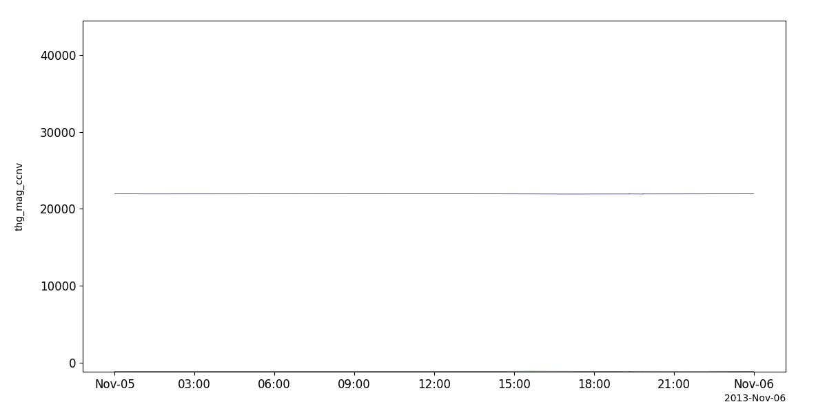
Example

import pyspedas
from pyspedas import tplot
gmag_vars = pyspedas.projects.themis.gmag(sites='ccnv', trange=['2013-11-5', '2013-11-6'])
tplot('thg_mag_ccnv')